For most of the history of electromagnetism, the potentials were understood as a convenience. Useful, often indispensable in practice, but not themselves part of the furniture of the world.
The reasoning was sound. Maxwell’s theory can be written entirely in terms of the electric and magnetic fields. Those are what push on a charge; those are what an instrument responds to. The potentials φ and A enter as mathematical scaffolding — quantities from which the fields can be derived by differentiation, and which make many calculations far easier than they would otherwise be. And as the previous article discussed, they are not even uniquely defined: infinitely many choices of potential describe the same physical situation. A quantity you can change at will without changing anything measurable does not look like a physical object.
In 1959 that position became untenable.
A field that is not there
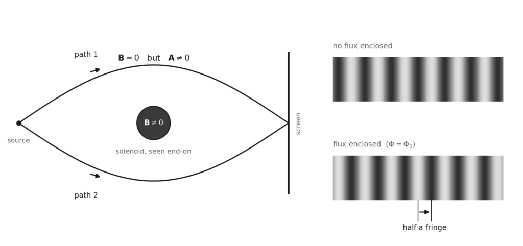
Consider a long solenoid — a tightly wound coil carrying a steady current. Inside it there is a magnetic field. Outside it, if the coil is long enough, there is essentially none: the field is confined to the interior.
The vector potential is a different matter. Outside the solenoid, where B vanishes, A does not. It circulates around the coil, falling off with distance but never reaching zero.
Classically this is of no consequence whatsoever. A charged particle passing outside the solenoid experiences no magnetic field, therefore no magnetic force, therefore nothing at all. The non-zero A in that region is exactly the sort of thing one expects of a gauge-dependent bookkeeping quantity: present in the mathematics, absent from the physics.
A classical counterpart of this geometry does exist, and is worth noting in passing. If the solenoid is driven with an alternating current, a conducting loop encircling it — but never entering it — develops a measurable electromotive force, even though the magnetic field along the loop is negligible. Faraday’s law in integral form accounts for this without difficulty, since it depends on the flux threading the circuit rather than on the field at the conductor. Rousseaux and co-workers, who studied the configuration theoretically and experimentally in 2008, named it the Maxwell–Lodge effect after an 1889 paper of Oliver Lodge, and argued that it is best understood in terms of the vector potential.
Two differences matter. The classical effect requires the current to vary in time; with a steady current there is no electromotive force and nothing to measure. And the field outside a real solenoid is small rather than exactly zero — a gap that would take decades to close for the quantum case.
What Yakir Aharonov and David Bohm proposed, in a paper published in Physical Review under the title Significance of Electromagnetic Potentials in the Quantum Theory, was that in quantum mechanics this is not true. An electron travelling through a region where the fields are rigorously zero is nonetheless affected by the potential, in a way that produces an observable consequence.
Why the potentials, and not the fields
The reason is structural, and it predates the effect by three decades. When electromagnetism is coupled to quantum mechanics, the fields do not appear in the equations at all. The potentials do.
The coupling is introduced by the minimal substitution: in the Hamiltonian of a particle of charge q, the momentum is replaced by the canonical momentum, and the scalar potential is added to the energy.
Written out, this is the operator that governs the evolution of the wavefunction:
There is no way to write this in terms of E and B. The Schrödinger equation for a charged particle is a statement about φ and A, and always was — a fact that attracted little comment for as long as everything it predicted could also be obtained from the fields.
Gauge invariance survives because a change of gauge multiplies the wavefunction by a position-dependent phase, which leaves every probability unchanged. But a phase that cancels in the modulus need not cancel between two interfering paths — and that is the whole of the effect.
How you would see it
The prediction concerns interference, so it is worth a sentence on what that means here.
An electron beam split into two paths and recombined produces a pattern of alternating light and dark bands — fringes — because the electron behaves as a wave, and the two halves of that wave arrive either in step or out of step depending on the difference in what they have encountered along the way. Shift the relative timing of the two halves, and the whole pattern slides sideways. The size of that shift is a measurement.
Now run one path on each side of the solenoid. Neither electron ever enters a region with a magnetic field. But the two paths, taken together, enclose the solenoid — and the phase difference between them is
where the integral runs around the closed loop formed by the two paths, and Φ is the magnetic flux threading it. The fringes shift, by an amount fixed by the flux inside a region the electrons never visited.
The part that is easy to state wrongly
It is tempting to summarise this as “the vector potential is physically real after all.” That is too quick, and the precise version is more interesting.
A is still not gauge-invariant. Change gauge and its value at any given point changes, exactly as before. What is gauge-invariant is the integral around a closed loop, because the extra term introduced by a gauge transformation is a gradient, and the integral of a gradient around any closed path vanishes identically:
So the observable is not A at a point. It is the loop integral — a global quantity, belonging to the path as a whole rather than to any location on it.
This has a consequence that is easy to miss. Whether the loop integral can be non-zero, in a region where the field vanishes, depends on the shape of the region. The solenoid geometry works because the electron paths enclose something they cannot enter: the accessible region has a hole in it. Given a region without such a hole — one in which every loop can be shrunk continuously to a point — a vanishing field forces the loop integral to vanish too, no matter how large A happens to be locally.
The requirement that the solenoid be long, which reads at first like an engineering detail, is doing exactly this work. It is what makes the exterior region topologically non-trivial.
1949
There is an earlier paper.
In 1949, Werner Ehrenberg and Raymond Siday published in the Proceedings of the Physical Society a study of the refractive index in electron optics which discusses a substantially equivalent effect — a decade before Aharonov and Bohm, in a journal nobody would have thought to overlook.
It went essentially unnoticed. The result was framed as a technical point within electron optics rather than as a statement about the status of the potentials, and it reached an audience of instrument specialists rather than of physicists interested in foundations. The effect is now occasionally called Ehrenberg–Siday–Aharonov–Bohm, which is accurate and which almost nobody says.
The pattern is the same one that swallowed Lorenz’s name, with a different mechanism. There the correct attribution lost to a more famous near-homophone. Here it lost to framing: the same physics, presented as a correction to a specialist calculation instead of as a challenge to a foundational assumption, simply did not register.
Closing the last gap
The prediction was contested for years, and the objection was a fair one. Real solenoids are finite. A small amount of magnetic field always leaks into the region the electrons traverse, and a sceptic could maintain that the observed shift was caused by that leakage rather than by the potential in a genuinely field-free region.
Settling it took until the 1980s, and the work of Akira Tonomura and his collaborators at Hitachi. Electron holography experiments in 1982 established the shift. The decisive experiment came in 1986.
They built a toroidal magnet roughly six micrometres across — a doughnut, so that the field lines close on themselves inside it with no ends to leak from — and then covered the whole thing in a superconducting shell. A superconductor expels magnetic field from its interior, the Meissner effect, so the shell acted as a barrier that no field line could cross. The magnetic field was not merely small outside the torus. It was excluded, by a mechanism independent of the geometry.
The observed fringe shift was exactly half a fringe — the value required by the quantisation of magnetic flux in a superconductor, in units of
Not approximately half. The number the theory demanded, produced by a system in which the alternative explanation had been physically eliminated.
What changed
The classical position was that the fields carry the physics and the potentials carry the bookkeeping. After 1986 that cannot be maintained. There is an experiment in which the fields are zero everywhere the particle goes, and something happens anyway.
What replaced it is not the opposite claim. A is not an ordinary field with a definite value at each point; it remains gauge-dependent, and any description that treats its pointwise value as measurable is wrong. What the experiments establish is narrower and stranger: that there exists a gauge-invariant quantity built from the potentials, not reducible to the fields, which is not local — it belongs to a closed path rather than to a place — and which nature is demonstrably sensitive to.
The potentials turned out not to be scaffolding. They turned out to be carrying something the field description had no way to express.
Sources
- W. Ehrenberg and R. E. Siday, “The Refractive Index in Electron Optics and the Principles of Dynamics,” Proc. Phys. Soc. London, vol. B62, p. 8, 1949.
- Y. Aharonov and D. Bohm, “Significance of Electromagnetic Potentials in the Quantum Theory,” Phys. Rev., vol. 115, pp. 485–491, 1959.
- A. Tonomura et al., “Observation of Aharonov-Bohm Effect by Electron Holography,” Phys. Rev. Lett., vol. 48, pp. 1443–1446, 1982.
- A. Tonomura et al., “Evidence for Aharonov-Bohm Effect with Magnetic Field Completely Shielded from Electron Wave,” Phys. Rev. Lett., vol. 56, pp. 792–795, 1986.
- N. Osakabe et al., “Experimental Confirmation of Aharonov-Bohm Effect Using a Toroidal Magnetic Field Confined by a Superconductor,” Phys. Rev. A, vol. 34, pp. 815–822, 1986.
- G. Rousseaux, R. Kofman, and O. Minazzoli, “The Maxwell-Lodge effect: significance of electromagnetic potentials in the classical theory,” Eur. Phys. J. D, vol. 49, pp. 249–256, 2008.
Leave a Reply