A conducting sphere is charged, and in the region outside it the electromagnetic field is exactly zero — no electric field, no magnetic field, no Poynting flux — for as long as the charging lasts. A receiver placed in that region nevertheless produces a measurable voltage, arriving at the speed of light.
The first half of that has been established elsewhere, along with the considerable qualifications it requires. This article is about the second half: what the receiver is responding to, given that there is nothing there to push its electrons around.
The route that leads nowhere
The obvious place to start is the classical equation of motion. A conductor responds to fields; write the force on a conduction electron and see what it gives.
It gives zero. The Lorentz force is the charge times the electric field plus the velocity cross the magnetic field, and both fields vanish. The equation is satisfied identically, for an electron of any velocity, at every point and every instant.
That is not a difficulty to be worked around. It is correct, and it is the whole content of the classical level: no force, no classical dynamics. An identity of the form nothing equals nothing determines nothing, and no amount of care in solving it will produce a mechanism.
So the classical equation of motion is the wrong instrument. It is not that it gives the wrong answer — it gives no answer, and says so honestly.
Where the coupling actually lives
The right instrument is the Hamiltonian, and the reason is worth stating in general terms before looking at this particular case.
The relation between a force balance and a Hamiltonian is the relation between statics and analytical mechanics. Knowing that the normal force on a block equals its weight tells you nothing about how a constrained system moves; the dynamics come from the Lagrangian or the Hamiltonian, and they contain terms that no force diagram displays. The same asymmetry applies here, and it is the standard structure of mechanics rather than anything peculiar to this problem.
Written out for a conduction electron in the Lorenz gauge, the minimal-coupling Hamiltonian is:
Four terms beyond the free kinetic energy. The last of them is the one that matters, and the crucial point about it is structural: the term involving the scalar potential is not part of the kinetic sector. It does not descend from the momentum operator, it is not what generates the Lorentz force, and it does not vanish when the fields vanish. It sits there as long as the potential is non-zero, whatever the fields are doing.
What it does, in a conductor, is shift the electrochemical potential:
uniformly across the receiver. Every conduction electron finds its energy reference displaced, in step, by an amount that tracks the potential in time.
What happened to the other three terms
This is where the argument could easily have gone wrong, and where checking it changes the answer.
Two of the remaining terms — the paramagnetic and the diamagnetic — are exactly the ones a bulk conductor usually picks up, and they involve the vector potential, which is emphatically not zero here. A first estimate, taking the paramagnetic term alone against a single-electron energy scale, suggested they might contribute a per cent or a few per cent of the response.
That estimate does not survive the correct treatment, and the reason it fails is instructive. In any bulk conduction response, gauge invariance of the conductivity — expressed through the f-sum rule, standard in linear response theory — forces the paramagnetic and diamagnetic terms to combine. They cannot appear separately in an observable. What they combine into is a response that depends only on the physical field:
and the physical field is identically zero throughout the dynamic regime. So the bulk conduction current is not one to four per cent. It is exactly zero — the same null result as at the classical level, now extended from the Lorentz force to the entire bulk-conduction channel, paramagnetic and diamagnetic terms included.
The estimate was superseded rather than confirmed, and the correction went in the direction of strengthening the null result rather than weakening it. Recording that matters more than the number: an approximate answer of one to four per cent and an exact answer of zero are different kinds of statement, and the second is the one that stands.
The fourth term, the non-Hermitian one, is bounded separately and comes out around one part in a million. It is not the mechanism either.
What the electrons respond to
That leaves the potential term, and the question of how it produces a current. Here the linear-response machinery has to be applied with some care, because the natural way to set it up gives nothing.
Standard practice couples the perturbation to the electric field and computes the current response. Do that here, in the long-wavelength limit appropriate to a receiver small compared to the distances involved, and the answer vanishes — consistently with the field being zero, and uselessly. That route is not wrong, it is empty. It cannot be used.
The physically correct route couples the perturbation to the charge density instead, which is to say to the potential itself rather than to its gradient. The response function obtained that way remains finite in the same limit. And the physical reading of that statement is the point of the whole exercise:
The electrons are not responding to a spatial gradient of the potential across the receiver. To leading order there is none — the potential is essentially uniform over the device. They are responding to the change in time of their own local electrochemical potential.
That is an ordinary mechanism. It is classical linear response of the Kubo–Drude kind, the same machinery used for conductivity in metals, with a relaxation time in the tens of femtoseconds — nine orders of magnitude faster than the transients involved. Nothing exotic is being invoked. What is unusual is only the perturbation it is being applied to.
The agent and the condition
One distinction deserves to be made explicit, because the two halves of it are easy to conflate and they are not the same statement.
The agent is the potential itself, not its rate of change. The coupling term in the Hamiltonian contains the potential, and it is present whenever the potential is non-zero, whether or not it is changing. A constant potential still shifts the electrochemical potential and still displaces the equilibrium charge distribution of the conductor accordingly.
What a constant potential does not do is sustain a current. The displaced distribution, once reached, is stationary — the conductor equilibrates to its new reference and then nothing further happens.
The rate of change enters only through continuity:
If the charge density at a point is changing, a current must flow. So a non-zero rate of change is what turns a one-off equilibration into a continuing, measurable current — the condition under which a receiver can register the effect, rather than a second mechanism competing with the first.
Two levels of the same physics: the coupling in the Hamiltonian, and the observability enforced by continuity. Not two rival explanations.
What the bookkeeping quantities are, and are not
A programme of this kind accumulates derived quantities — a scalar built from the divergence of the vector potential, an energy density formed from it, a flux, several integrated energies. It is worth being blunt about their status, because the temptation to promote them is real and the discipline against it is what keeps the account honest.
None of them is independent physical energy, flux, or radiated power.
The scalar quantity itself is gauge-dependent by construction: it vanishes identically in Coulomb gauge, which is enough to settle the question on its own. The energy density and flux built from it are local diagnostics, and where they are non-trivial the ordinary electromagnetic stress-energy tensor is identically zero — so there is nothing for them to be carrying. Several of the integrated quantities numerically anticipate a physical energy, which is a useful property and not the same as being one. Others turn out to be local re-expressions of circuit power that has already been counted once at the terminals; counting it twice would be an error, not a discovery.
Exactly one quantity in the family is physical field energy, and it is the settled electrostatic energy after the transient is over.
What all the others share is a single common status, and it is better stated once than corrected six times: they are gauge-dependent diagnostics of where and when the physical process is active — that process being the potential coupling in the Hamiltonian, and nothing else. A diagnostic that tells you accurately when something is happening is worth having. It is not the thing that is happening.
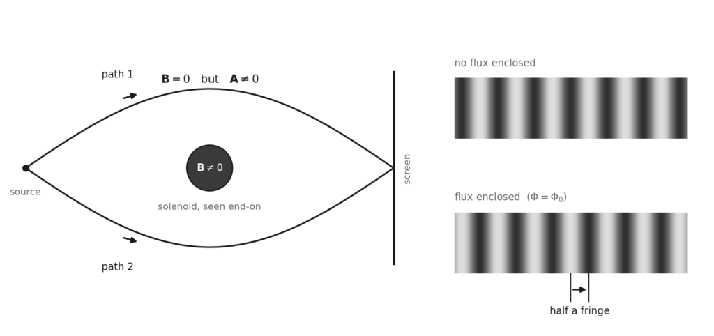
Not an Aharonov–Bohm effect
The comparison is unavoidable and should be made carefully, because the resemblance is real and the identification would be wrong.
Aharonov and Bohm established that a potential can have observable consequences in a region where the gauge-invariant field vanishes. That principle is what is at work here too, and the debt should be acknowledged.
But the scalar version of their effect requires the electric field to vanish at the location of the charge, which is achieved with a Faraday-shielded enclosure, and the observable is a quantum phase shift measured by interference. Here the geometry is open and unshielded, a particular field quantity at the receiver is not zero, and the mechanism is classical linear response producing a terminal voltage — no interference, no phase measurement, no shielding.
Same principle, different mechanism. Not a macroscopic reproduction, and describing it as one would be an overstatement that the details do not support.
What remains open
One structural question in this account is not settled. The construction of the vector potential used throughout is argued to be the unique causal one consistent with the source and the gauge condition, but the argument is presented informally rather than as a proof. A formal demonstration combining the causality requirement with the multipole selection rule has not been given.
Until it is, the correct description is that the construction is well motivated and consistent, not that it is unique. The distinction matters, and marking it is cheaper than defending it later.