Immediately

A bar of metal lies in empty space with its axis along a uniform external electric field. At some moment the field is switched on. What happens inside the metal?

The standard answer is three words long. Charges redistribute, and a field appears inside the conductor that immediately cancels the external one, leaving the interior field-free.

Every part of that is true. The word carrying the weight is immediately, and it is hiding four separate physical processes whose characteristic times differ by twelve orders of magnitude. Two of them are not what the sentence leads you to expect, and one of them is usually calculated in a way that contradicts its own assumptions.

The setup, precisely

Numbers are only meaningful against a stated configuration, so here is the one used throughout.

The bar is AISI 430 ferritic stainless steel, 4 mm in diameter and 10 cm long, isolated in vacuum, electrically neutral, with no connection to anything. Its conductivity is taken as 1.7 × 10⁶ S/m and its carrier density as 1.7 × 10²⁹ per cubic metre, both nominal figures for a ferritic steel rather than measurements of a particular sample.

The applied field is weak: weak enough that any magnetic flux density arising anywhere in the problem stays well below 0.5 T, comfortably short of the saturation of this material and within the region where the permeability can be treated as a constant. The relative permeability is therefore the low-field value, taken as lying somewhere between 200 and 1000; a range is quoted rather than a single number because permeability is not a material constant but a property of the working point, and the maximum-of-curve values that appear on datasheets belong to a different regime from this one.

The bar is isolated and neutral throughout. Nothing is earthed, no current leaves it, and no load is connected. The external field polarises it and nothing more: positive charge gathers at one end, an equal negative charge at the other, and the total remains zero.

That last point matters more than it may seem, and we will return to it.

The number that is quoted

The screening time of a conductor is derived in essentially every course, and the derivation takes three lines. Ohm’s law in its instantaneous form, the continuity equation, and Gauss’s law:

Combining them gives an exponential decay of any excess charge density, with time constant

For the bar described above this is 5.2 × 10⁻¹⁸ seconds. The conclusion drawn is that charge redistribution in a good conductor is, for all practical purposes, instantaneous.

The derivation is correct. Each step follows from the one before, and as an exercise it tests exactly what it means to test. The difficulty is with the number it produces.

Why that number cannot mean what it says

This steel has an electron collision time of about 3.5 × 10⁻¹⁶ seconds. The screening time just derived is roughly seventy times shorter than that.

This should stop us. The instantaneous form of Ohm’s law is a statement that the current density responds to the field with no delay, and that statement is an approximation valid only when nothing in the problem changes appreciably within one collision time. The derivation has produced a process that completes in a small fraction of a collision time — which is to say, it has produced a result lying far outside the domain where its own first premise holds.

There is a second warning. The plasma period of this material is 2.7 × 10⁻¹⁶ seconds. The quoted screening time is shorter than that too, by a factor of about fifty. Below the plasma period the electron gas has not had time to complete a single collective oscillation, and treating it as a resistive medium is not meaningful.

So the result invalidates its own assumptions twice over. This is a different kind of error from a mistake in algebra, and a more interesting one: a formally correct derivation delivering an answer outside its region of validity, with nothing in the derivation itself to signal that this has happened.

What replaces it

The repair is small. Keep Gauss and continuity, and replace the instantaneous Ohm’s law with the simplest form that acknowledges the electrons have inertia — the Drude relation, in which the current density relaxes towards its ohmic value over the collision time rather than reaching it at once:

This is the first term beyond instantaneous response, and it is the classical limit of the linear-response treatment of conduction. Combining it with the same two equations as before gives, for the excess charge density,

which is not an exponential decay at all. It is a damped harmonic oscillator, with natural frequency the plasma frequency and damping rate set by the collision time.

Everything now depends on a single dimensionless number: the product of the collision time and a frequency. The frequency in question is not quite the bare plasma frequency but the longitudinal frequency, the one at which the dielectric function vanishes once the high-frequency interband response is folded in. It is smaller than the plasma frequency by the square root of that response.

When the product of longitudinal frequency and collision time falls below one half the oscillator is overdamped, and its slow root is exactly the textbook result: the standard answer is recovered, in the regime where it belongs. Above one half the oscillator is underdamped, and the excess charge does not decay monotonically. It rings.

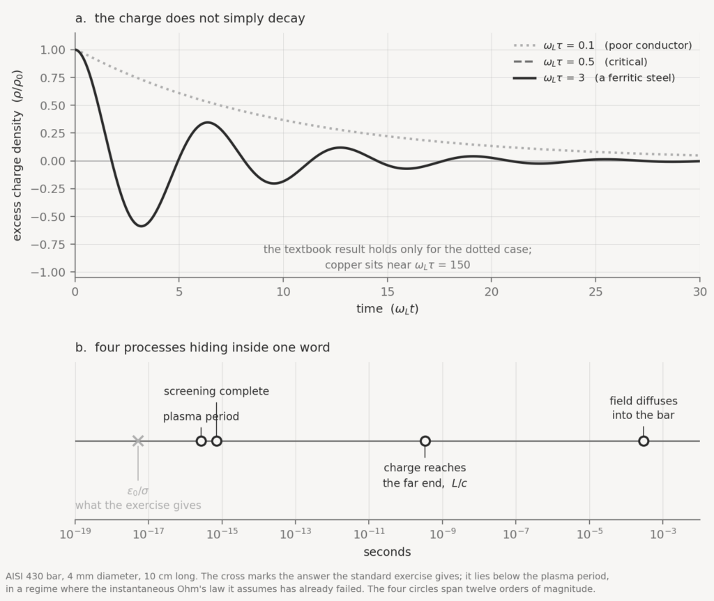
For this steel the product is somewhere between two and four. The uncertainty is honest: the interband response of a ferritic steel is not a figure I have found tabulated, and it enters under a square root. But the classification does not depend on resolving it. Any value in that range is several times the threshold, and even a very large interband response would not bring the material below it.

So excess charge in this bar does not sink quietly to zero in 5.2 × 10⁻¹⁸ seconds. It oscillates while decaying, and the decay takes about 7.1 × 10⁻¹⁶ seconds, twice the collision time. The ratio between the true relaxation time and the textbook one is twice the square of the dimensionless number, so of order twenty here.

A ferritic steel is chosen because it is a poor conductor as metals go, and therefore the least favourable metal for this argument. Better conductors are further from the textbook regime, not closer. Copper sits near 150; measured values for lead and gold are about 9 and 57 respectively. No metal is in the regime where the textbook derivation applies. What is in that regime is a lightly doped semiconductor, where the product is well below one half and the exact treatment agrees with the classical formula closely.

The formula is not wrong. It is being evaluated outside its house.

None of this is new

It is worth saying plainly that the correction above is not a discovery, and I am not the first to notice it. The failure of the textbook relaxation time in good conductors has been pointed out in the pedagogical literature at least since Saslow and Wilkinson in 1971, again by Ashby in 1975, and worked out in full in a recent monograph on dielectric response by Riffe, who observes that the naive result implies a charge density relaxing faster than the fundamental relaxation time of the very carriers that carry it, and calls that conclusion nonsense.

That the point has been made repeatedly across fifty years and still does not appear where the formula is taught is the interesting part. It is not a controversy. It is a correction that has never found its way into the exercise.

The charge has to travel

Set all of that aside; it concerns what happens at one point in the metal. There is a second process, and it is geometric rather than material.

The interior field is cancelled by surface charge, and that surface charge has to accumulate somewhere. For a bar along the field it accumulates at the two ends, positive at one and negative at the other. Those ends are ten centimetres apart, and no rearrangement can propagate between them faster than light.

For a bar ten centimetres long this is 3.3 × 10⁻¹⁰ seconds. It is six orders of magnitude slower than the local screening, and it is set entirely by the length of the bar — the conductivity of the metal does not enter it at all. However good the conductor, the far end cannot learn what the near end is doing before a light-transit time has elapsed.

So the field-free interior is not established everywhere at once. It is established locally, very fast, and globally at a rate limited by the geometry.

How the two fit together

It is worth being explicit about how these processes combine, because a list invites the reader to hear a sequence, and a sequence is the wrong picture.

The local screening and the light-transit time are not consecutive stages of the same journey. They operate on different levels. At every point in the metal the electron gas responds to whatever field it finds there, and it does so within a few femtoseconds; but what field it finds there depends on where the charge has already moved, and that information cannot travel faster than light.

The result is a front. Switch the external field on, and the near end of the bar begins accumulating charge at once. That charge sets up its own field, which propagates outward. A point in the middle of the bar knows nothing of it until light has covered the distance, and until then that point sits in the applied field with no correction. Once the front arrives, the local response is essentially instantaneous on the scale of the front’s motion, and the interior field there collapses.

What sweeps along the bar is therefore not the charge and not the screening, but the boundary between the region that has adjusted and the region that has not. Behind it, the interior field is already zero. Ahead of it, the metal is still unaware anything has happened. The bar becomes field-free progressively, from the ends inward, at a rate set by the speed of light and not by the conductivity.

Even this is a simplification: the front is not sharp, the geometry of a real bar makes the propagation more complicated than a single sweep, and there is a settling period after the first transit during which the charge distribution converges on its final form through several reflections. But the essential picture is right, and it is different from the one the three-word answer suggests. Nothing about the process is instantaneous. What is fast is the local response; what is slow, relatively speaking, is the conversation between the two ends.

The fourth process, the magnetic diffusion, is not part of this sequence at all. It concerns a different field, arises from the currents that flow during the transient rather than from the applied field, and continues long after the electric screening is complete. It is included in the count because it too hides inside the word immediately, not because it belongs to the same chain of events.

It radiates

The charge migrating to the ends of the bar is a current, flowing for a fraction of a nanosecond along a definite path. A transient current in a definite spatial pattern radiates, and a bar with charge accumulating at its two ends is, for the duration of the transient, an elementary dipole.

This is worth pausing on, because it is entirely absent from the three-word account. An object described as passively shielding itself is, during the transient, an antenna. The fields it emits are weak and brief, and in most circumstances nobody cares — but they are not zero, and they cannot be made zero by choosing a better conductor, because the radiation is a consequence of the shape and the time scale rather than of the material.

It also turns out to be the thing that ends the transient.

The bar is open at both ends, so as far as the transient is concerned it is a short transmission line terminated in an open circuit at each end. The reflection coefficient at an open end is plus one. The disturbance that starts at the near end travels to the far end, reflects without inversion, comes back, reflects again. Nothing about the geometry stops it.

Something has to remove the energy, and there are only two candidates: heating the metal, or radiating. The two can be compared. At the frequencies involved — the round trip along a 10 cm bar corresponds to about 1.5 GHz — the skin depth in this steel is around 10 micrometres, so the current is confined to a thin surface layer and the effective resistance per metre is roughly a hundred times its direct-current value. That sounds significant, and it is not: the resulting damping corresponds to a quality factor in the low thousands, which is to say thousands of round trips. Radiation, by contrast, gives a quality factor of order ten. It dominates by something like three orders of magnitude.

So the bar settles because it radiates, not because it is resistive. A hypothetical conductor that could not radiate would ring for thousands of transits, in any metal.

How long that takes depends on where one draws the line, since an exponential never reaches zero. Taking one per cent of the initial amplitude as the threshold gives roughly nine round trips, or about six nanoseconds for the bar described here. This is not a precise figure. At a quality factor of order ten the damping is strong enough that talk of distinct reflections is already a loose way of speaking — the disturbance deforms as it travels rather than returning intact — and counting round trips is itself a high-quality-factor approximation being used where it does not strictly apply. What is robust is the comparison between the two loss channels, not the number of bounces.

The important structural point is that this all happens in the skin. During the settling the current lives in ten micrometres of surface, and the interior of the bar takes no part in it. The same permeability and the same conductivity govern both the skin depth and the diffusion time discussed below, through the same physics at opposite ends of the spectrum: at the frequencies of the ringing the field does not enter the metal at all, and at the frequencies of the slow transient it enters completely, but slowly.

The magnetic field has to get in, or out

The fourth process is the slowest by far.

Inside a conductor the electromagnetic field does not propagate. It diffuses, governed by an equation of the same form as heat conduction: drop the displacement current from the Ampere-Maxwell law, substitute Ohm, and what remains is

For a cylinder the fundamental mode decays with a time constant equal to the permeability times the conductivity times the square of the radius, divided by the square of the first zero of the Bessel function J0, which is 5.78. Note the radius squared: halving the diameter divides this time by four.

For the bar described at the start, with the permeability somewhere in the low-field range assumed, this comes out between about 300 microseconds and 1.5 milliseconds.

That is six orders of magnitude slower than the light-transit time along the bar, nearly five orders of magnitude slower than the electrical settling described above, and twelve orders of magnitude slower than the local screening. The same object screens locally in femtoseconds and takes hundreds of microseconds to let a magnetic field into its interior — because the two are entirely different physical processes wearing the same word.

Two qualifications belong here, and both are in the spirit of the rest of this article. The expression is the fundamental mode for an infinitely long cylinder in an axial field, so for a bar of finite length it is an order-of-magnitude estimate rather than an exact result. Note also that the corresponding constant for a slab of thickness d is the same expression with the square of pi in place of the Bessel factor; the two geometries are often quoted interchangeably and they are not the same. And iron is not linear: treating the permeability as a constant is what makes the diffusion equation solvable, and it is legitimate only in the weak-field regime stated at the outset. In a real ferromagnetic bar the flux front advances as a switching zone rather than a smooth exponential, and hysteresis losses add to the eddy-current losses. The time constant gives the scale correctly; it does not give the waveform.

This is also the reason a conducting body is an excellent electrostatic screen and a mediocre magnetic one, a distinction familiar to anyone who has designed an enclosure and mysterious to anyone who has only read the three-word account. Iron inverts the usual ranking, too: it is a far worse conductor than copper and a far better magnetic screen, precisely because the high permeability that slows the diffusion is what makes it useful. Woodson and Melcher make the same observation in their treatment of magnetic diffusion, noting that silicon iron has a longer diffusion time than copper despite a conductivity more than an order of magnitude lower, and that this is why iron cores must be laminated in alternating-current equipment.

A remark about closed loops

Everything above concerns a bar: an open shape, with two ends. It is worth asking what changes if the ends are joined.

Bend the bar into a ring and the answer changes in a way that is exact rather than approximate. The electromotive force driving current round the loop is the line integral of the electric field around it. Writing the field in terms of the scalar and vector potentials, the scalar contribution is the closed line integral of a gradient, and that vanishes identically for any single-valued potential:

What remains is the vector potential term, which is the rate of change of magnetic flux through the loop.

So the two shapes respond to different things. The bar polarises because charge piles up at its ends, and the field that cancels the applied one inside the metal is the gradient of a scalar potential — that term does all the work. Close the bar into a ring and that same term contributes exactly nothing, and what is left responds only to changing flux.

This is not an approximation for slow fields, nor a statement about a particular choice of gauge. It follows from the topology of the path: the circulation of a gradient around any closed curve is zero, whatever the potentials are doing. A closed loop is blind to one whole part of the description of the field, by construction, and detecting that part at all requires a path that does not close.

Which returns to the stipulation made at the beginning, that the bar is isolated and neutral with nothing connected to it. The charge separation is real and the potential difference between the ends is real, but with no external path there is nowhere for that separation to do anything. It establishes itself and stops. An open shape can respond to the scalar part; whether that response is available for anything depends on what, if anything, is attached to the ends.

What the exercise is really teaching

None of this makes the standard treatment useless. For nearly every purpose the interior of a good conductor is field-free, immediately, and the three-word account is the right thing to say.

But the exercise as usually set does something worth noticing. It asks the student to combine three equations correctly, which they do, and then hands them a number to interpret, which they cannot — because interpreting it requires knowing the collision time and the plasma frequency, quantities the exercise never mentions. The result carries no warning that it has left the domain of its own assumptions, and there is nothing in the calculation that could supply one.

The general lesson is not about conductors. Every constitutive relation is an approximation with a domain, and the algebra that uses it will not tell you when you have stepped outside. Instantaneous Ohm’s law assumes nothing changes within a collision time; use it to compute something faster than a collision time and it will still return an answer, formatted like all the others, with no indication that it means nothing.

Sources

• N. W. Ashcroft and N. D. Mermin, Solid State Physics. New York: Holt, Rinehart and Winston, 1976, Ch. 1.
• W. M. Saslow and G. Wilkinson, “Expulsion of free electronic charge from the interior of a metal,” Am. J. Phys., vol. 39, pp. 1244-1246, 1971.
• N. Ashby, “Relaxation of charge imbalances in conductors,” Am. J. Phys., vol. 43, pp. 553-555, 1975.
• D. M. Riffe, “Canonical Models of Dielectric Response,” arXiv:1806.05158, 2018, Sec. 8.
• H. H. Woodson and J. R. Melcher, Electromechanical Dynamics. New York: Wiley, 1968, Ch. 7.
• J. D. Jackson, Classical Electrodynamics, 3rd ed. New York: Wiley, 1998, Ch. 5 and 7.
• H. E. Knoepfel, Magnetic Fields: A Comprehensive Theoretical Treatise for Practical Use. New York: Wiley, 2000, Ch. 4.
• Material figures are nominal values for a ferritic stainless steel, not measurements: conductivity 1.7 x 10^6 S/m, carrier density 1.7 x 10^29 per cubic metre, low-field relative permeability taken as 200 to 1000. Collision time and plasma frequency follow from the first two by the Drude relations, and every ratio quoted in the text is reproducible from them.