Category: Forgotten Topics

  • Neither Field Creates the Other

    What the causal solution of Maxwell’s equations actually says

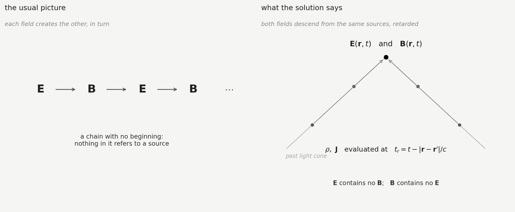
    Almost every introduction to electromagnetic waves tells the same story. A changing electric field produces a magnetic field; that magnetic field, also changing, produces an electric field; and the two, taking turns, hand energy back and forth as the disturbance propagates away. It is a vivid picture, it appears in textbooks and lecture courses everywhere, and it makes the wave feel like something that sustains itself once launched.

    There is a way of writing the solution of Maxwell’s equations in which that picture does not appear at all. In it, the electric field at a point contains no reference to the magnetic field anywhere, and the magnetic field contains no reference to the electric one. Both are written entirely in terms of charges and currents, evaluated at earlier times. Nothing takes turns with anything.

    The equations are usually named after Oleg Jefimenko, who published them in 1966. Whether the picture they displace is wrong, or merely not forced, turns out to be a more delicate question than either side of the argument usually admits — and the delicate part is where this article ends up.

    What the causal solution looks like

    Maxwell’s equations in differential form relate fields and sources at a single instant. The curl equations in particular put a time derivative of one field on one side and the other field on the other side, both evaluated now:

    ∇×𝐄=−∂𝐁∂t,∇×𝐁=μ0𝐉+μ0ε0∂𝐄∂t\nabla \times \mathbf{E} = -\frac{\partial \mathbf{B}}{\partial t}, \qquad \nabla \times \mathbf{B} = \mu_{0}\mathbf{J} + \mu_{0}\varepsilon_{0}\frac{\partial \mathbf{E}}{\partial t}

    Read as a statement of what causes what, this is already strange. The two sides are simultaneous. Whatever relation holds between them, it is not one in which the right-hand side has had time to bring the left-hand side about, because no time has passed at all. Jefimenko put the point bluntly: since each of these equations connects quantities simultaneous in time, none of them can represent a causal relation.

    The solution of the same equations, for an arbitrary distribution of charge and current, can be written so that the time structure is explicit. Two pieces of shorthand keep it readable: R for the vector from a source point to the point of observation, and a dot for a time derivative. The retarded time follows from the first:

    𝐑=𝐫−𝐫′,R=|𝐑|,𝐑^=𝐑/R,tr=t−R/c\mathbf{R} = \mathbf{r}-\mathbf{r}’, \qquad R = |\mathbf{R}|, \qquad \hat{\mathbf{R}} = \mathbf{R}/R, \qquad t_{r} = t – R/c

    That is, the moment early enough that a signal leaving the source point then, travelling at c, arrives at the observation point now. Every source quantity in what follows — ρ, J, and their time derivatives — is evaluated at that earlier moment, never at the observation time. With that understood, the electric field is

    𝐄(𝐫,t)=14πε0∫[ρ𝐑^R2+ρ˙𝐑^cR−𝐉˙c2R]d3r′\mathbf{E}(\mathbf{r},t) = \frac{1}{4\pi\varepsilon_{0}} \int \left[ \frac{\rho\,\hat{\mathbf{R}}}{R^{2}} + \frac{\dot{\rho}\,\hat{\mathbf{R}}}{cR} – \frac{\dot{\mathbf{J}}}{c^{2}R} \right] d^{3}r’

    and the magnetic field

    𝐁(𝐫,t)=μ04π∫[𝐉R2+𝐉˙cR]×𝐑^d3r′\mathbf{B}(\mathbf{r},t) = \frac{\mu_{0}}{4\pi} \int \left[ \frac{\mathbf{J}}{R^{2}} + \frac{\dot{\mathbf{J}}}{cR} \right] \times \hat{\mathbf{R}}\; d^{3}r’

    Two features of these expressions do the work, and both are visible without evaluating a single integral.

    The first is that the right-hand sides are in the past. Not simultaneous, not implicitly retarded, but explicitly evaluated at an earlier instant fixed by the light travel time. Whatever the sources were doing then determines what the fields are here now.

    The second is what is missing. The expression for E contains ρ and J and their time derivatives. It does not contain B. The expression for B contains J and its time derivative. It does not contain E. Neither field appears in the other’s formula, at any time, retarded or otherwise. Jefimenko’s own conclusion follows directly: the electromagnetic field is a dual entity, always having an electric and a magnetic component, simultaneously created by their common sources — time-varying charges and currents.
    Why they are locked together in the far field

    There is an obvious objection, and it is worth meeting head-on. Far from any source, the two fields are not merely correlated but rigidly tied: the magnetic field is perpendicular to the electric one and to the direction of propagation, with magnitudes in the fixed ratio

    𝐁=1c𝐑^×𝐄\mathbf{B} = \frac{1}{c}\,\hat{\mathbf{R}} \times \mathbf{E}

    That is about as tight a relationship as two quantities can have. If neither field has anything to do with the other, why do they march in lockstep?

    The answer is visible in the expressions themselves, once one asks which terms survive at large distance. Of the three contributions to E, the first falls off as 1/R² and is negligible far away; the two carrying time derivatives of the sources fall only as 1/R and are what remains. Charge conservation then does something specific: the longitudinal part of the current-derivative term cancels exactly against the charge-derivative term, and what is left is the transverse part of the current derivative alone. In the expression for B, the surviving 1/R term is that same current derivative, crossed with R̂ — which selects precisely the same transverse quantity.

    Written out, with J̇⊥ for the part of the current derivative perpendicular to the line of sight, the two radiation fields are:

    𝐄rad=−μ04π∫𝐉˙⟂Rd3r′,𝐁rad=μ04πc∫𝐉˙⟂×𝐑^Rd3r′\mathbf{E}_{\text{rad}} = -\frac{\mu_{0}}{4\pi} \int \frac{\dot{\mathbf{J}}_{\perp}}{R}\, d^{3}r’, \qquad \mathbf{B}_{\text{rad}} = \frac{\mu_{0}}{4\pi c} \int \frac{\dot{\mathbf{J}}_{\perp} \times \hat{\mathbf{R}}}{R}\, d^{3}r’

    So in the radiation zone both fields reduce to integrals over one and the same thing: the transverse acceleration of charge at the retarded time. One of them carries an extra cross product with the line of sight, and that is the entire difference between them. The fixed ratio and the mutual perpendicularity follow from that by algebra, not by any influence passing between them.

    This is a common-cause correlation, and the distinction is not a quibble. Two quantities descending from the same ancestor can be rigidly related without either producing the other — and the structure here shows exactly that pattern, because the lockstep holds only where both expressions collapse onto the shared term. Closer in, where the 1/R² contributions are still present, the ratio of the field magnitudes is not c, the two are not in phase, and the neat orthogonality fails. Any mechanism by which one field genuinely generated the other would have to operate everywhere, not only in the region where the two formulas happen to reduce to the same integral.

    The far-field relation, in other words, is the strongest-looking evidence for the mutual-induction picture, and on inspection it is evidence against it.

    Where they come from

    Nothing new is being introduced. These are Maxwell’s equations, solved, and the route is short.

    Start from the retarded potentials in Lorenz gauge — the same objects, and the same gauge condition, discussed elsewhere on this site:

    φ(𝐫,t)=14πε0∫ρRd3r′,\varphi(\mathbf{r},t) = \frac{1}{4\pi\varepsilon_{0}}\int \frac{\rho}{R}\, d^{3}r’,
    𝐀(𝐫,t)=μ04π∫𝐉Rd3r′\mathbf{A}(\mathbf{r},t) = \frac{\mu_{0}}{4\pi}\int \frac{\mathbf{J}}{R}\, d^{3}r’

    Then substitute the definitions of the fields in terms of the potentials, and differentiate under the integral sign. The derivatives act on the retarded time as well as on the explicit distance dependence, which is where the extra terms in 1/R and 1/R² come from. What emerges is the pair above.

    This matters for how much weight the result can carry. Jefimenko’s equations are not an alternative theory, a modification, or a reinterpretation. They are the general solution of the standard equations, written in one particular way. Anything true of them is true of Maxwell’s electrodynamics; the question is only what becomes visible in this form that was hidden in the other.

    Who wrote them first

    The attribution is tangled in a way that will be familiar to anyone who has followed the Lorenz and Ehrenberg–Siday cases discussed elsewhere here.

    David Griffiths, whose textbook is where most physicists meet these expressions, is careful about it: the earliest explicit statement of which he is aware was Jefimenko’s, in 1966. Kirk McDonald has pointed out that time-domain expressions of essentially this form appear four years earlier, in the second edition of Panofsky and Phillips’s Classical Electricity and Magnetism of 1962, where the electric field is written in a slightly different but entirely equivalent form. And the closely related formula for the fields of a single point charge in arbitrary motion — often called the Heaviside–Feynman formula — was published by Oliver Heaviside in 1904, then rediscovered by Feynman and presented in the Lectures in 1963, apparently without knowledge of the earlier result.

    Three independent arrivals, spanning six decades, at expressions that were available in principle from the moment the retarded potentials were understood. The pattern is the one this site keeps running into: the mathematics was not the obstacle. What was missing each time was a reason to write the solution in that particular form, and an audience for whom the form mattered.

    Jefimenko’s contribution, on the evidence, was less the derivation than the insistence on what it meant. Panofsky and Phillips wrote the expressions and moved on. Jefimenko spent decades arguing about them.

    What this does not settle

    Here the argument needs slowing down, because the strong version of the claim is repeated more often than it is examined, and it does not survive contact with two facts.

    Retardation was chosen, not derived

    The retarded solution is not the only solution of Maxwell’s equations. There is also an advanced one, identical in form except that the sources are evaluated at

    ta=t+Rct_{a} = t + \frac{R}{c}

    — that is, in the future. It satisfies the same equations exactly as well. The full general solution is any combination of the two, plus a source-free solution of the homogeneous equation.

    Choosing the retarded solution alone is a physical input, made on the grounds that fields should propagate outward from sources rather than converge inward from infinity. It is a boundary condition, and a well-motivated one, but it is not a consequence of Maxwell’s equations. So the causal structure that Jefimenko’s form displays so clearly was, in a precise sense, put in by hand at the moment the retarded Green’s function was selected.

    This does not make the equations wrong or the argument empty. It relocates it. The equations do not prove that sources cause fields rather than fields causing each other; they show that once the ordinary radiation boundary condition is imposed, the solution can be written entirely in terms of sources, with no field-on-field dependence anywhere. That is a genuine structural fact about the theory, and it is not what the mutual-induction story leads one to expect.

    The equations describe fields produced by given sources, and nothing else

    The second limitation is stated in the equations’ own preamble and is easy to read past. They give the fields produced by an assigned distribution of charge and current, on the assumption that there is no electromagnetic field present other than the one those sources produce.

    A plane wave crossing empty space with no sources anywhere is a perfectly good solution of Maxwell’s equations, and Jefimenko’s expressions have nothing to say about it: with ρ and J set to zero, both integrals vanish, and one is left with the source-free solution that had to be added separately. The same applies to a field in a resonant cavity long after whatever excited it has been switched off.

    So the claim cannot be that no electromagnetic field ever exists without sources. It is narrower: that the fields of a given source distribution are determined by that distribution alone, with the two components arising together rather than one generating the other.

    The dispute is live

    None of this is settled interpretation. Jefimenko’s causal reading was challenged directly in the pages of the American Journal of Physics — Rohrlich argued in 2002 that the Coulomb field’s causal status does not work the way Jefimenko’s programme requires, Jefimenko replied in the same volume, and Rohrlich replied again. Reasonable physicists disagree about how much metaphysical weight a choice of Green’s function can bear.

    What is not in dispute is the mathematics. Everyone agrees the expressions are correct solutions of Maxwell’s equations, and everyone can see that E does not appear in the formula for B.

    The same point, seen in another algebra

    The argument above was made by comparing two expressions and observing what each one lacks. There is a formalism in which the observation needs no comparison, because the two fields are not two objects to begin with.

    In the biquaternion formulation used throughout this site — in One Operator, Four Domains and The Fifth Equation — the potentials and the sources are each a single object, scalar part imaginary and vector part real:

    A~=[𝐢cφ,𝐀],\tilde{A} = \left[ \frac{\mathbf{i}}{c}\varphi, \; \mathbf{A} \right], \qquad
    J~=[𝐢cρ,𝐉]\tilde{J} = \left[ \mathbf{i}c\rho, \; \mathbf{J} \right]

    Applying the operator twice gives the whole inhomogeneous system in one line, the wave equations for both potentials at once:

    ∇~2A~=μ0J~\tilde{\nabla}^{2} \tilde{A} = \mu_{0} \tilde{J}

    And applying it once to the potential gives the fields — not two expressions to be compared, but the two slots of a single result:

    2∇~A~=B~−𝐢cE~,2\tilde{\nabla}\tilde{A} = \tilde{B} – \frac{\mathbf{i}}{c}\tilde{E}, \qquad
    b≡∇⋅𝐀=−1c2∂φ∂tb \equiv \nabla \cdot \mathbf{A} = -\frac{1}{c^{2}}\frac{\partial \varphi}{\partial t}

    The vector slot carries both fields together, 2B − (2i/c)E; the scalar slot carries the Lorenz quantity b.

    Written this way, the point of this article stops being an inference and becomes a feature of the notation. One does not check that E fails to appear in the formula for B, because there is no separate formula for either: there is one object, produced by one operation acting on one retarded source. That the two components arise together, from a common ancestor, is not a conclusion drawn from inspecting the solution — it is what the solution is.

    The far-field relation reads the same way. If the fields are two slots of one object, the rigid tie between them at large distance is a condition on that object, not a negotiated agreement between two independent entities. The transverse structure that emerged above from cancellation between terms is, in this language, a statement about what survives in the vector slot at order 1/R.

    One further remark belongs here, because it bears on what this article has been arguing. That same single application also fills the scalar slot — with the Lorenz condition, as developed at length in The Fifth Equation. The gauge condition is not an auxiliary constraint bolted on to four field equations; it arrives with them, from the same operation. That matters in the present context, because the retarded solution used throughout this article is the Lorenz-gauge one, and the causal structure everything here depends on is inseparable from that choice.

    The same algebra has been developed independently outside this programme, in different conventions: Gsponer writes Maxwell’s inhomogeneous system as a single biquaternion equation for a field bivector, and takes the construction back through Paul Weiss’s quaternionic radiation theory of 1941 to Hamilton himself. The notation differs — Gaussian units, c = 1, the fields carried as a bivector rather than in the slots used here — but the structure is the same one, and readers coming from that literature will recognise it.

    Nothing in this section is a new result, and no claim of one is intended: this is the same solution of the same equations, written in an algebra that happens to make one of its features conspicuous. But that is worth something on its own. A formalism in which a true statement is hard to see, and another in which it is hard to miss, are not equally good descriptions of the same physics — and which of the two is the standard one is a matter of history rather than of merit.

    What survives

    The useful residue is smaller than the strongest claims made for these equations, and more solid.

    The mutual-induction story is a picture attached to a particular way of writing the equations, not a fact the equations assert. Written in the form above, the same theory offers no support for it at all: two fields, both descending from the same sources at the same retarded time, neither making any reference to the other.

    It is worth being fair about where that picture comes from, because it is not arbitrary. In Heaviside’s local form — the differential equations as every course presents them — the curl of E genuinely is tied to the rate of change of B, and the curl of B to the rate of change of E. As a statement about constraint, that reading is correct: given one field, the other is not free. The two are rigidly linked at every point, and the local equations are exactly where one sees it.

    What the local form cannot show is why they are linked. A constraint between two quantities is equally well explained by one producing the other and by both descending from a common ancestor, and nothing in the differential equations distinguishes the two — not least because, as Jefimenko pointed out, their two sides are simultaneous, so neither has had time to bring the other about. The retarded form settles what the local form leaves open: the ancestor is there, in the sources, and the constraint is what remains of it.

    So the slippage is a narrow one, and easy to make. A student told that a changing E creates a B which creates an E has been handed a correct description of a constraint, relabelled as a mechanism.

    Whether that mnemonic is harmless is a matter of taste, but it has a cost worth noting. It suggests that a wave, once launched, sustains itself by an internal exchange — and therefore that something about the wave is doing work to keep it going. Jefimenko’s form makes clear that nothing needs to sustain anything: the field at a distant point now is simply what the sources were doing at the retarded time, propagated outward, with no bootstrapping required.

    That is a modest result. But it is the kind of modesty that follows from writing the same thing a second way and looking at what changed — which, in a subject where the standard formalism has been fixed for over a century, is one of the few remaining ways to learn something about it.


    Sources

    • O. D. Jefimenko, Electricity and Magnetism: An Introduction to the Theory of Electric and Magnetic Fields. New York: Appleton-Century-Crofts, 1966; 2nd ed., Star City: Electret Scientific, 1989.
    • O. D. Jefimenko, Causality, Electromagnetic Induction, and Gravitation, 2nd ed. Star City: Electret Scientific, 2000, ch. 1 (source of the quoted remarks on simultaneity and on the dual nature of the field).
    • W. K. H. Panofsky and M. Phillips, Classical Electricity and Magnetism, 2nd ed. Reading, MA: Addison-Wesley, 1962, sec. 14.3.
    • K. T. McDonald, “The relation between expressions for time-dependent electromagnetic fields given by Jefimenko and by Panofsky and Phillips,” Am. J. Phys., vol. 65, no. 11, pp. 1074–1076, 1997.
    • D. J. Griffiths and M. A. Heald, “Time-dependent generalizations of the Biot–Savart and Coulomb laws,” Am. J. Phys., vol. 59, no. 2, pp. 111–117, 1991.
    • D. J. Griffiths, Introduction to Electrodynamics, 3rd ed. Upper Saddle River: Prentice Hall, 1999, pp. 427–438.
    • O. Heaviside, Electromagnetic Theory, vol. 3, 1904 (point-charge field formula); R. P. Feynman, R. B. Leighton and M. Sands, The Feynman Lectures on Physics, vol. 1, 1963, sec. 28-1.
    • A. Gsponer, “Derivation of the potential, field, and locally-conserved charge-current density of an arbitrarily moving point-charge,” ISRI-06-04, arXiv:physics/0612232 (biquaternion treatment of the retarded point-charge field).
    • P. Weiss, “On some applications of quaternions to restricted relativity and classical radiation theory,” Proc. Roy. Irish Acad., vol. 46, pp. 129–168, 1941.
    • A. Gsponer and J.-P. Hurni, “The physical heritage of Sir W. R. Hamilton,” arXiv:math-ph/0201058.
    • F. Rohrlich, “Causality, the Coulomb field, and Newton’s law of gravitation,” Am. J. Phys., vol. 70, pp. 411–414, 2002; O. D. Jefimenko, comment, and F. Rohrlich, reply, Am. J. Phys., vol. 70, p. 964, 2002.
  • Immediately

    A bar of metal lies in empty space with its axis along a uniform external electric field. At some moment the field is switched on. What happens inside the metal?

    The standard answer is three words long. Charges redistribute, and a field appears inside the conductor that immediately cancels the external one, leaving the interior field-free.

    Every part of that is true. The word carrying the weight is immediately, and it is hiding four separate physical processes whose characteristic times differ by twelve orders of magnitude. Two of them are not what the sentence leads you to expect, and one of them is usually calculated in a way that contradicts its own assumptions.

    The setup, precisely

    Numbers are only meaningful against a stated configuration, so here is the one used throughout.

    The bar is AISI 430 ferritic stainless steel, 4 mm in diameter and 10 cm long, isolated in vacuum, electrically neutral, with no connection to anything. Its conductivity is taken as 1.7 × 10⁶ S/m and its carrier density as 1.7 × 1029 per cubic metre, both nominal figures for a ferritic steel rather than measurements of a particular sample.

    The applied field is weak: weak enough that any magnetic flux density arising anywhere in the problem stays well below 0.5 T, comfortably short of the saturation of this material and within the region where the permeability can be treated as a constant. The relative permeability is therefore the low-field value, taken as lying somewhere between 200 and 1000; a range is quoted rather than a single number because permeability is not a material constant but a property of the working point, and the maximum-of-curve values that appear on datasheets belong to a different regime from this one.

    The bar is isolated and neutral throughout. Nothing is earthed, no current leaves it, and no load is connected. The external field polarises it and nothing more: positive charge gathers at one end, an equal negative charge at the other, and the total remains zero.

    That last point matters more than it may seem, and we will return to it.

    The number that is quoted

    The screening time of a conductor is derived in essentially every course, and the derivation takes three lines. Ohm’s law in its instantaneous form, the continuity equation, and Gauss’s law:

    𝐉=σ𝐄,∇⋅𝐉+∂ρ∂t=0,∇⋅𝐄=ρε0\mathbf{J} = \sigma \mathbf{E}, \qquad \nabla \cdot \mathbf{J} + \frac{\partial \rho}{\partial t} = 0, \qquad \nabla \cdot \mathbf{E} = \frac{\rho}{\varepsilon_0}

    Combining them gives an exponential decay of any excess charge density, with time constant

    ∂ρ∂t=−σε0ρ⟹τM=ε0σ\frac{\partial \rho}{\partial t} = -\frac{\sigma}{\varepsilon_0} \rho \qquad \Longrightarrow \qquad \tau_M = \frac{\varepsilon_0}{\sigma}

    For the bar described above this is 5.2 × 10⁻¹⁸ seconds. The conclusion drawn is that charge redistribution in a good conductor is, for all practical purposes, instantaneous.

    The derivation is correct. Each step follows from the one before, and as an exercise it tests exactly what it means to test. The difficulty is with the number it produces.

    Why that number cannot mean what it says

    This steel has an electron collision time of about 3.5 × 10⁻¹⁶ seconds. The screening time just derived is roughly seventy times shorter than that.

    This should stop us. The instantaneous form of Ohm’s law is a statement that the current density responds to the field with no delay, and that statement is an approximation valid only when nothing in the problem changes appreciably within one collision time. The derivation has produced a process that completes in a small fraction of a collision time — which is to say, it has produced a result lying far outside the domain where its own first premise holds.

    There is a second warning. The plasma period of this material is 2.7 × 10⁻¹⁶ seconds. The quoted screening time is shorter than that too, by a factor of about fifty. Below the plasma period the electron gas has not had time to complete a single collective oscillation, and treating it as a resistive medium is not meaningful.

    So the result invalidates its own assumptions twice over. This is a different kind of error from a mistake in algebra, and a more interesting one: a formally correct derivation delivering an answer outside its region of validity, with nothing in the derivation itself to signal that this has happened.

    What replaces it

    The repair is small. Keep Gauss and continuity, and replace the instantaneous Ohm’s law with the simplest form that acknowledges the electrons have inertia — the Drude relation, in which the current density relaxes towards its ohmic value over the collision time rather than reaching it at once:

    τ∂𝐉∂t+𝐉=σ0𝐄\tau \frac{\partial \mathbf{J}}{\partial t} + \mathbf{J} = \sigma_0 \mathbf{E}

    This is the first term beyond instantaneous response, and it is the classical limit of the linear-response treatment of conduction. Combining it with the same two equations as before gives, for the excess charge density,

    ∂2ρ∂t2+1τ∂ρ∂t+ωL2ρ=0,ωL=ωpε∞,ωp2=ne2ε0m\frac{\partial^2 \rho}{\partial t^2} + \frac{1}{\tau} \frac{\partial \rho}{\partial t} + \omega_L^2 \rho = 0, \qquad \omega_L = \frac{\omega_p}{\sqrt{\varepsilon_\infty}}, \qquad \omega_p^2 = \frac{n e^2}{\varepsilon_0 m}

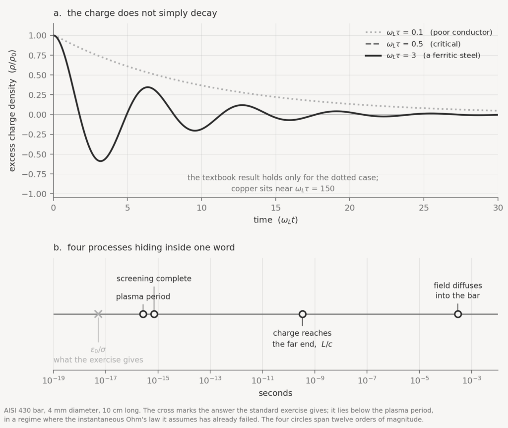
    which is not an exponential decay at all. It is a damped harmonic oscillator, with natural frequency the plasma frequency and damping rate set by the collision time.

    Everything now depends on a single dimensionless number: the product of the collision time and a frequency. The frequency in question is not quite the bare plasma frequency but the longitudinal frequency, the one at which the dielectric function vanishes once the high-frequency interband response is folded in. It is smaller than the plasma frequency by the square root of that response.

    When the product of longitudinal frequency and collision time falls below one half the oscillator is overdamped, and its slow root is exactly the textbook result: the standard answer is recovered, in the regime where it belongs. Above one half the oscillator is underdamped, and the excess charge does not decay monotonically. It rings.

    For this steel the product is somewhere between two and four. The uncertainty is honest: the interband response of a ferritic steel is not a figure I have found tabulated, and it enters under a square root. But the classification does not depend on resolving it. Any value in that range is several times the threshold, and even a very large interband response would not bring the material below it.

    So excess charge in this bar does not sink quietly to zero in 5.2 × 10⁻¹⁸ seconds. It oscillates while decaying, and the decay takes about 7.1 × 10⁻¹⁶ seconds, twice the collision time. The ratio between the true relaxation time and the textbook one is twice the square of the dimensionless number, so of order twenty here.

    A ferritic steel is chosen because it is a poor conductor as metals go, and therefore the least favourable metal for this argument. Better conductors are further from the textbook regime, not closer. Copper sits near 150; measured values for lead and gold are about 9 and 57 respectively. No metal is in the regime where the textbook derivation applies. What is in that regime is a lightly doped semiconductor, where the product is well below one half and the exact treatment agrees with the classical formula closely.

    The formula is not wrong. It is being evaluated outside its house.

    None of this is new

    It is worth saying plainly that the correction above is not a discovery, and I am not the first to notice it. The failure of the textbook relaxation time in good conductors has been pointed out in the pedagogical literature at least since Saslow and Wilkinson in 1971, again by Ashby in 1975, and worked out in full in a recent monograph on dielectric response by Riffe, who observes that the naive result implies a charge density relaxing faster than the fundamental relaxation time of the very carriers that carry it, and calls that conclusion nonsense.

    That the point has been made repeatedly across fifty years and still does not appear where the formula is taught is the interesting part. It is not a controversy. It is a correction that has never found its way into the exercise.

    The charge has to travel

    Set all of that aside; it concerns what happens at one point in the metal. There is a second process, and it is geometric rather than material.

    The interior field is cancelled by surface charge, and that surface charge has to accumulate somewhere. For a bar along the field it accumulates at the two ends, positive at one and negative at the other. Those ends are ten centimetres apart, and no rearrangement can propagate between them faster than light.

    For a bar ten centimetres long this is 3.3 × 10⁻¹⁰ seconds. It is six orders of magnitude slower than the local screening, and it is set entirely by the length of the bar — the conductivity of the metal does not enter it at all. However good the conductor, the far end cannot learn what the near end is doing before a light-transit time has elapsed.

    So the field-free interior is not established everywhere at once. It is established locally, very fast, and globally at a rate limited by the geometry.

    How the two fit together

    It is worth being explicit about how these processes combine, because a list invites the reader to hear a sequence, and a sequence is the wrong picture.

    The local screening and the light-transit time are not consecutive stages of the same journey. They operate on different levels. At every point in the metal the electron gas responds to whatever field it finds there, and it does so within a few femtoseconds; but what field it finds there depends on where the charge has already moved, and that information cannot travel faster than light.

    The result is a front. Switch the external field on, and the near end of the bar begins accumulating charge at once. That charge sets up its own field, which propagates outward. A point in the middle of the bar knows nothing of it until light has covered the distance, and until then that point sits in the applied field with no correction. Once the front arrives, the local response is essentially instantaneous on the scale of the front’s motion, and the interior field there collapses.

    What sweeps along the bar is therefore not the charge and not the screening, but the boundary between the region that has adjusted and the region that has not. Behind it, the interior field is already zero. Ahead of it, the metal is still unaware anything has happened. The bar becomes field-free progressively, from the ends inward, at a rate set by the speed of light and not by the conductivity.

    Even this is a simplification: the front is not sharp, the geometry of a real bar makes the propagation more complicated than a single sweep, and there is a settling period after the first transit during which the charge distribution converges on its final form through several reflections. But the essential picture is right, and it is different from the one the three-word answer suggests. Nothing about the process is instantaneous. What is fast is the local response; what is slow, relatively speaking, is the conversation between the two ends.

    The fourth process, the magnetic diffusion, is not part of this sequence at all. It concerns a different field, arises from the currents that flow during the transient rather than from the applied field, and continues long after the electric screening is complete. It is included in the count because it too hides inside the word immediately, not because it belongs to the same chain of events.

    It radiates

    The charge migrating to the ends of the bar is a current, flowing for a fraction of a nanosecond along a definite path. A transient current in a definite spatial pattern radiates, and a bar with charge accumulating at its two ends is, for the duration of the transient, an elementary dipole.

    This is worth pausing on, because it is entirely absent from the three-word account. An object described as passively shielding itself is, during the transient, an antenna. The fields it emits are weak and brief, and in most circumstances nobody cares — but they are not zero, and they cannot be made zero by choosing a better conductor, because the radiation is a consequence of the shape and the time scale rather than of the material.

    It also turns out to be the thing that ends the transient.

    The bar is open at both ends, so as far as the transient is concerned it is a short transmission line terminated in an open circuit at each end. The reflection coefficient at an open end is plus one. The disturbance that starts at the near end travels to the far end, reflects without inversion, comes back, reflects again. Nothing about the geometry stops it.

    Something has to remove the energy, and there are only two candidates: heating the metal, or radiating. The two can be compared. At the frequencies involved — the round trip along a 10 cm bar corresponds to about 1.5 GHz — the skin depth in this steel is around 10 micrometres, so the current is confined to a thin surface layer and the effective resistance per metre is roughly a hundred times its direct-current value. That sounds significant, and it is not: the resulting damping corresponds to a quality factor in the low thousands, which is to say thousands of round trips. Radiation, by contrast, gives a quality factor of order ten. It dominates by something like three orders of magnitude.

    So the bar settles because it radiates, not because it is resistive. A hypothetical conductor that could not radiate would ring for thousands of transits, in any metal.

    How long that takes depends on where one draws the line, since an exponential never reaches zero. Taking one per cent of the initial amplitude as the threshold gives roughly nine round trips, or about six nanoseconds for the bar described here. This is not a precise figure. At a quality factor of order ten the damping is strong enough that talk of distinct reflections is already a loose way of speaking — the disturbance deforms as it travels rather than returning intact — and counting round trips is itself a high-quality-factor approximation being used where it does not strictly apply. What is robust is the comparison between the two loss channels, not the number of bounces.

    The important structural point is that this all happens in the skin. During the settling the current lives in ten micrometres of surface, and the interior of the bar takes no part in it. The same permeability and the same conductivity govern both the skin depth and the diffusion time discussed below, through the same physics at opposite ends of the spectrum: at the frequencies of the ringing the field does not enter the metal at all, and at the frequencies of the slow transient it enters completely, but slowly.

    The magnetic field has to get in, or out

    The fourth process is the slowest by far.

    Inside a conductor the electromagnetic field does not propagate. It diffuses, governed by an equation of the same form as heat conduction: drop the displacement current from the Ampere-Maxwell law, substitute Ohm, and what remains is

    ∇2𝐁=μσ∂𝐁∂t,τd=μσa2j012,j01≃2.405\nabla^2 \mathbf{B} = \mu \sigma \frac{\partial \mathbf{B}}{\partial t}, \qquad \tau_d = \frac{\mu \sigma a^2}{j_{01}^2}, \quad j_{01} \simeq 2.405

    For a cylinder the fundamental mode decays with a time constant equal to the permeability times the conductivity times the square of the radius, divided by the square of the first zero of the Bessel function J0, which is 5.78. Note the radius squared: halving the diameter divides this time by four.

    For the bar described at the start, with the permeability somewhere in the low-field range assumed, this comes out between about 300 microseconds and 1.5 milliseconds.

    That is six orders of magnitude slower than the light-transit time along the bar, nearly five orders of magnitude slower than the electrical settling described above, and twelve orders of magnitude slower than the local screening. The same object screens locally in femtoseconds and takes hundreds of microseconds to let a magnetic field into its interior — because the two are entirely different physical processes wearing the same word.

    Two qualifications belong here, and both are in the spirit of the rest of this article. The expression is the fundamental mode for an infinitely long cylinder in an axial field, so for a bar of finite length it is an order-of-magnitude estimate rather than an exact result. Note also that the corresponding constant for a slab of thickness d is the same expression with the square of pi in place of the Bessel factor; the two geometries are often quoted interchangeably and they are not the same. And iron is not linear: treating the permeability as a constant is what makes the diffusion equation solvable, and it is legitimate only in the weak-field regime stated at the outset. In a real ferromagnetic bar the flux front advances as a switching zone rather than a smooth exponential, and hysteresis losses add to the eddy-current losses. The time constant gives the scale correctly; it does not give the waveform.

    This is also the reason a conducting body is an excellent electrostatic screen and a mediocre magnetic one, a distinction familiar to anyone who has designed an enclosure and mysterious to anyone who has only read the three-word account. Iron inverts the usual ranking, too: it is a far worse conductor than copper and a far better magnetic screen, precisely because the high permeability that slows the diffusion is what makes it useful. Woodson and Melcher make the same observation in their treatment of magnetic diffusion, noting that silicon iron has a longer diffusion time than copper despite a conductivity more than an order of magnitude lower, and that this is why iron cores must be laminated in alternating-current equipment.

    A remark about closed loops

    Everything above concerns a bar: an open shape, with two ends. It is worth asking what changes if the ends are joined.

    Bend the bar into a ring and the answer changes in a way that is exact rather than approximate. The electromotive force driving current round the loop is the line integral of the electric field around it. Writing the field in terms of the scalar and vector potentials, the scalar contribution is the closed line integral of a gradient, and that vanishes identically for any single-valued potential:

    ∮𝐄⋅d𝐥=−∮∇φ⋅d𝐥−∮∂𝐀∂t⋅d𝐥=−dΦBdt\oint \mathbf{E} \cdot d\mathbf{l} = -\oint \nabla \varphi \cdot d\mathbf{l} – \oint \frac{\partial \mathbf{A}}{\partial t} \cdot d\mathbf{l} = -\frac{d\Phi_B}{dt}

    What remains is the vector potential term, which is the rate of change of magnetic flux through the loop.

    So the two shapes respond to different things. The bar polarises because charge piles up at its ends, and the field that cancels the applied one inside the metal is the gradient of a scalar potential — that term does all the work. Close the bar into a ring and that same term contributes exactly nothing, and what is left responds only to changing flux.

    This is not an approximation for slow fields, nor a statement about a particular choice of gauge. It follows from the topology of the path: the circulation of a gradient around any closed curve is zero, whatever the potentials are doing. A closed loop is blind to one whole part of the description of the field, by construction, and detecting that part at all requires a path that does not close.

    Which returns to the stipulation made at the beginning, that the bar is isolated and neutral with nothing connected to it. The charge separation is real and the potential difference between the ends is real, but with no external path there is nowhere for that separation to do anything. It establishes itself and stops. An open shape can respond to the scalar part; whether that response is available for anything depends on what, if anything, is attached to the ends.

    What the exercise is really teaching

    None of this makes the standard treatment useless. For nearly every purpose the interior of a good conductor is field-free, immediately, and the three-word account is the right thing to say.

    But the exercise as usually set does something worth noticing. It asks the student to combine three equations correctly, which they do, and then hands them a number to interpret, which they cannot — because interpreting it requires knowing the collision time and the plasma frequency, quantities the exercise never mentions. The result carries no warning that it has left the domain of its own assumptions, and there is nothing in the calculation that could supply one.

    The general lesson is not about conductors. Every constitutive relation is an approximation with a domain, and the algebra that uses it will not tell you when you have stepped outside. Instantaneous Ohm’s law assumes nothing changes within a collision time; use it to compute something faster than a collision time and it will still return an answer, formatted like all the others, with no indication that it means nothing.

    Sources

    • N. W. Ashcroft and N. D. Mermin, Solid State Physics. New York: Holt, Rinehart and Winston, 1976, Ch. 1.
    • W. M. Saslow and G. Wilkinson, “Expulsion of free electronic charge from the interior of a metal,” Am. J. Phys., vol. 39, pp. 1244-1246, 1971.
    • N. Ashby, “Relaxation of charge imbalances in conductors,” Am. J. Phys., vol. 43, pp. 553-555, 1975.
    • D. M. Riffe, “Canonical Models of Dielectric Response,” arXiv:1806.05158, 2018, Sec. 8.
    • H. H. Woodson and J. R. Melcher, Electromechanical Dynamics. New York: Wiley, 1968, Ch. 7.
    • J. D. Jackson, Classical Electrodynamics, 3rd ed. New York: Wiley, 1998, Ch. 5 and 7.
    • H. E. Knoepfel, Magnetic Fields: A Comprehensive Theoretical Treatise for Practical Use. New York: Wiley, 2000, Ch. 4.
    • Material figures are nominal values for a ferritic stainless steel, not measurements: conductivity 1.7 x 10^6 S/m, carrier density 1.7 x 10^29 per cubic metre, low-field relative permeability taken as 200 to 1000. Collision time and plasma frequency follow from the first two by the Drude relations, and every ratio quoted in the text is reproducible from them.
  • The Missing Half

    Charge a capacitor to V. Disconnect it. Now connect it, through a switch, to a second identical capacitor that is empty. Close the switch.

    Charge is conserved, and by symmetry it ends up shared equally, so both capacitors settle at half the original voltage. That much is uncontroversial and takes one line.

    Now count the energy. Before: one capacitor at V, holding half CV2. After: two capacitors, each at V/2, each holding a quarter of half CV2, for a total of one quarter CV2. Exactly half the energy has gone missing.

    The usual reaction is that this is a schoolroom trick and the answer is friction — some resistance somewhere ate it. That reaction is correct and also completely inadequate, because the interesting thing about this problem is not that energy is lost. It is how much, and what that quantity does not depend on.

    The resistor is not the culprit

    Put a resistor R in the connecting loop and do the integral.

    The two capacitors in series present C/2, so the loop time constant is RC/2. The current starts at V/R and decays exponentially. The energy delivered to the resistor is the integral of i2R, which comes to

    WR=∫0∞i2Rdt=V2R⋅RC4=14CV2W_R = \int_0^\infty i^2 R \, dt = \frac{V^2}{R} \cdot \frac{RC}{4} = \frac{1}{4} C V^2

    and R has cancelled. It is not there. Double the resistance and the current halves while the transient lasts twice as long; the square of the current falls by four and the duration rises by two, and the product is fixed.

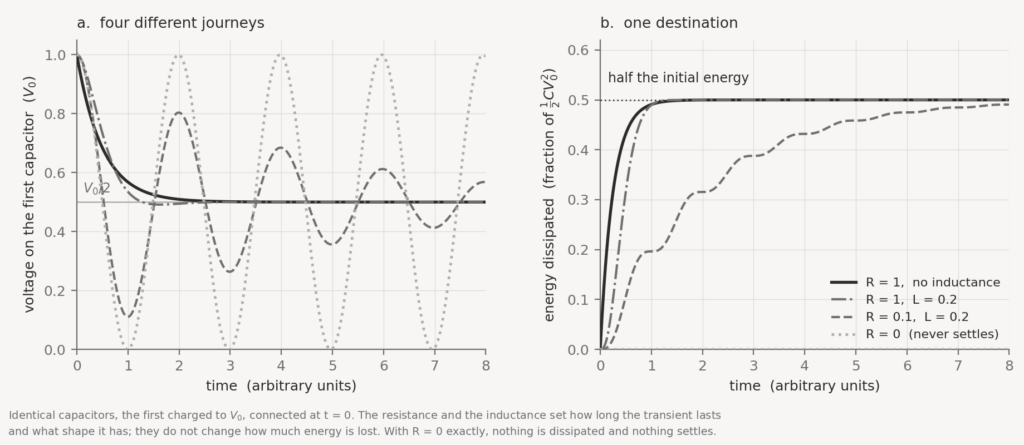
    So the missing quarter of CV2 is not a property of the connecting wire. It is fixed entirely by where the charge started and where it ended. The resistor is not the cause of the loss; it is merely the place where the loss happens to be deposited, and it will accept exactly the amount required of it whatever its value.

    This is worth restating because it inverts the usual intuition. One expects a lossy component to determine how much is lost. Here the loss is determined first, by the endpoints alone, and the component only reveals where it went.

    The general case

    Nothing about this depends on the capacitors being equal. Take two capacitors of any values at any voltages and connect them. Charge conservation fixes the common final voltage as the charge-weighted average, and the energy that disappears is

    ΔW=12⋅C1C2C1+C2(V1−V2)2\Delta W = \frac{1}{2} \cdot \frac{C_1 C_2}{C_1 + C_2} (V_1 – V_2)^2

    The prefactor is the series combination of the two capacitances, and the loss goes as the square of the initial voltage difference. It vanishes only when the two are already at the same voltage — that is, when nothing happens. Any transfer of charge between two capacitors at different potentials costs energy, and the cost is set before the transfer begins.

    Taking the resistance away

    If R never appears in the answer, what happens when we set it to zero?

    The formula still says a quarter of CV2 is lost, and now there is nothing to lose it to. This is the point at which the problem stops being a trick and becomes a real question.

    The first thing to notice is that a loop of wire with no resistance still has inductance, and inductance changes the story completely. With L in the circuit the charge does not simply flow across and stop. It overshoots. The system is a series LC resonator and the charge sloshes back and forth between the two capacitors, the first one emptying past the halfway point, refilling, emptying again.

    With any resistance at all, however small, the oscillation is damped and the system does eventually settle at the shared voltage — and the total dissipated over the whole ringing transient is again exactly a quarter of CV2. Not approximately: exactly, and independently of both R and L. The route changes completely; the destination does not.

    With R exactly zero and L greater than zero, something else happens: the oscillation never decays. There is no final state. The first capacitor returns periodically to its full initial voltage, and the energy is never lost because the system never arrives anywhere.

    This is the cleanest resolution of the paradox as usually posed, and it deserves to be stated plainly. The premise smuggles in the answer. Saying that the capacitors “end up” at V/2 is already an assumption that the transient dies, and a transient can only die by depositing its energy somewhere. Ask where half the energy went, having assumed a final state, and you have assumed the dissipation you are then surprised to find.

    And with no inductance either

    One can press further. Suppose the loop had neither resistance nor inductance — no ringing and no heating. Then where?

    At this point the lumped-circuit description has been asked for more than it can give. A loop with genuinely zero inductance would have to enclose no area, and a loop enclosing no area is not a circuit. Any real arrangement of two capacitors and a switch occupies space, and while the charge is redistributing it is accelerating, and accelerating charge radiates.

    The radiated fraction is negligible in any ordinary bench experiment, which is why nobody notices it and why the textbook answer of “the resistance” is a perfectly good practical answer. But it is not zero, and it cannot be made zero by improving the components, because it is a consequence of the geometry rather than of the materials. Radiation resistance is a property of shape. The idealisation that removes both R and L is the one that has left physics, not the one that has found a paradox in it.

    What the problem is actually about

    The structure here is worth separating from the specific circuit, because it recurs.

    There is a class of results in which a quantity is fixed by the initial and final states alone, while the mechanism that produces it is left entirely free. The energy lost in redistributing charge between capacitors is one. It does not care whether the loss occurs in a resistor, in the damping of an oscillation, or in radiated fields; it does not care how long any of that takes. The bookkeeping is settled in advance and the physics is left to find a channel.

    The same theorem, in a more familiar dress, governs charging a capacitor from a battery through a resistor. The battery delivers CV2. The capacitor keeps half of it and the resistor burns the other half — for any R, again with R cancelling out of the integral. Every capacitor charged from a fixed voltage source through a dissipative path wastes exactly half of what the source supplied, and no choice of component improves it. This is not a small fact. It is the reason a switching converter exists rather than a resistor.

    The two-capacitor problem is the same statement with the battery removed, and it looks paradoxical only because taking the battery away also removes the obvious place for the energy to go.

    The radiated fraction is negligible in any ordinary bench experiment, which is why nobody notices it and why the textbook answer of “the resistance” is a perfectly good practical answer. But it is not zero, and it cannot be made zero by improving the components, because it is a consequence of the geometry rather than of the materials. Radiation resistance is a property of shape. The idealisation that removes both R and L is the one that has left physics, not the one that has found a paradox in it.

    Where the energy goes, and why it has no choice

    Poynting’s theorem settles the destination as firmly as the endpoints settled the amount. Any decrease in the electromagnetic energy stored in a region has exactly two ways out: work done on charges, which in a resistor becomes heat, and flux through the boundary, which is radiation. There is no third term.

    So the missing quarter of CV2 is not merely lost — it is distributed between two channels, and which one collects it depends on the connecting loop rather than on the capacitors.

    With a substantial resistance, the transient is slow, the currents never accelerate sharply, and the loop is a hopeless antenna. Radiation is negligible and the resistor takes essentially all of it.

    With no resistance at all, heating is unavailable, and the balance has to be met some other way. The residual inductance makes the charge oscillate instead of settling, and an oscillating current in a loop of finite size radiates. The wires can be twisted to cancel the field in their immediate neighbourhood, but the cancellation cannot be exact everywhere, because the two conductors are not in the same place and their contributions arrive at a distant point with different delays. So the loop radiates, weakly, and goes on radiating until the oscillation has died — by which time exactly a quarter of CV2 has left as electromagnetic waves.

    The two extremes pay in different currency and the invoice is identical.

    There is something worth noticing in that. The electrons do not know the answer in advance. Each one responds only to the field where it is, at the instant it is there, with no knowledge of the final state. Yet the total comes out fixed. Nothing is coordinating them — the amount was determined by where the charge started and where it ended, and every route between those two points, however it is arranged, costs the same.

    Sources

    • W. K. H. Panofsky and M. Phillips, Classical Electricity and Magnetism, 2nd ed. Reading, MA: Addison-Wesley, 1962.
    • J. D. Jackson, Classical Electrodynamics, 3rd ed. New York: Wiley, 1998, Ch. 6.
    • The numerical results and the figure in this article are reproducible from first principles; the transient is the standard series RLC loop with two capacitors, integrated directly.