An instrument produces a reading. Before the reading means anything, one question has to be answered: what is the instrument responding to?
It is a harder question than it looks, and it is not answered by knowing how the instrument works. A coil of wire near a switching source will produce a voltage, and it will produce one whether the coupling is magnetic induction, capacitive pickup along the leads, a ground loop through the oscilloscope, or something else. The reading is the same in every case. An ordinary coil responds to everything, which is another way of saying it distinguishes nothing.
The way out is not a better measurement. It is a differently shaped instrument: one built to be blind to the things that are not of interest, so that whatever survives can be attributed. This article is about such a receiver — what makes it selective, and what four independent tests establish about the signal it registers.
Cancelling the magnetic channel
The receiver is a bifilar coil: two parallel conductors wound together along the same path, carrying current in opposite directions. Twenty-five double turns of 0.3 mm enamelled copper on a PVC tube, 1.7 cm across and 25 cm long, with 3 mm between conductors and a 1 cm pitch.
The winding is a standard technique for a standard reason. Two adjacent conductors carrying opposed currents enclose almost no net area, so the flux linked by the pair very nearly cancels, and with it the electromotive force that a changing magnetic field would otherwise induce. Bifilar windings are used wherever inductance is unwanted — in precision resistors, for instance.
Here the motivation is inverted. The suppression is not a convenience but the point of the exercise: the coil is wound this way in order to remove one candidate explanation from the field. Whatever it registers, magnetic induction is not a live account of it.
Screening is a property of topology
The second property of the receiver is the one that is easy to miss, and it is the one that makes it work.
A conductor placed in an external potential does not screen because it is made of copper. It screens because its charges can rearrange into a configuration that cancels the potential inside — and that rearrangement requires somewhere to rearrange to. A closed surface provides it. The induced charges distribute themselves over the enclosure, the interior potential goes flat, and nothing further happens. This is the Faraday cage, and its essential ingredient is the closure, not the metal.
A bifilar coil has two terminals and no closed surface. The charges still move — they must, because their energy reference has shifted — but there is no configuration available to them that cancels the effect. The only route open is toward the terminals. That motion is a current, and a current across a load is a voltage.
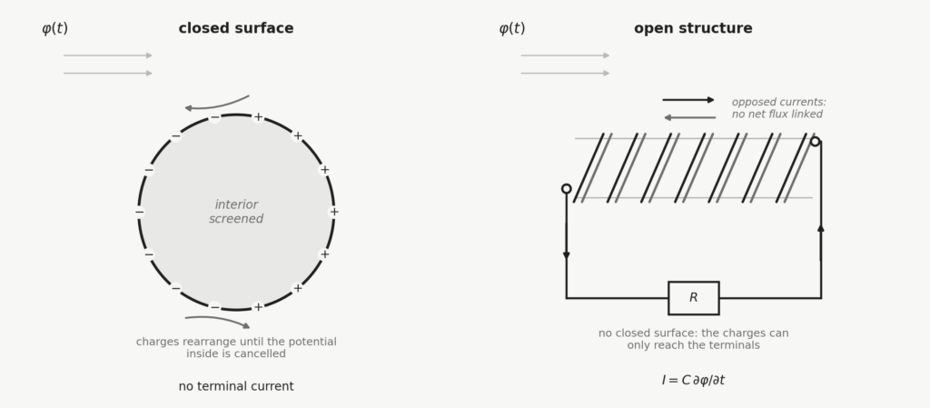
Put compactly: the conductor attempts to screen, the attempt cannot complete, and the failure is the signal. The terminal current takes the form
where the capacitance measures how strongly the structure couples to a potential it has no way of expelling. The microscopic account of why conduction electrons respond to a potential at all, in a region where the gauge-invariant fields vanish, is a separate matter and is treated in another article. What matters here is the geometry.
A capacitance that is predicted, not fitted
The coupling capacitance is the sort of quantity that can absorb a discrepancy if it is allowed to. Left as a free parameter it will fit almost anything, and a model that fits by adjustment establishes very little.
It can be estimated instead. The self-capacitance of a single circular loop of wire follows from its radius and the wire gauge — about 0.43 pF per turn for this geometry — and twenty-five turns give a geometric total near 32 pF. The differential winding roughly halves the coupling, since the two conductors of each pair partly shield one another. The prediction is about 15 pF.
The measured geometric capacitance, extracted from the resonance of the receiver circuit with the probe contribution removed, is about 15 pF. The number was not adjusted to make anything agree.
The first test: internal impedance
Varying the load resistance across seven decades, from 0.1 Ω to 1 MΩ, makes the receiver behave as a voltage divider, and the resistance at which the output falls to half its maximum gives the internal impedance of the source. The measurement returns 377 ± 10 Ω.
That number is the impedance of free space, 376.73 Ω, which sits 0.07 per cent from the central value and comfortably inside the interval. Capacitive pickup would not give it: at the operating frequency the reactance of the estimated mutual capacitance is around 4000 Ω, an order of magnitude away. The two hypotheses are not close enough to be confused.
It is worth being clear about what the free-space impedance does and does not indicate. It is the ratio μ₀c, fixed by the propagation speed alone, and it is therefore not a signature of any particular polarisation — a wave travelling at c will present it whatever its mode. Measuring 377 Ω is evidence about a speed, not about a geometry.
The second test: propagation velocity
The speed can also be measured directly, which is the more demanding version of the same question. Twenty-five independent time-delay readings were taken at a separation of 50 cm, triggering on the transmitter channel and timing the arrival at the receiver.
The sample mean is 3.049 × 10⁸ m/s, with a standard deviation of 1.575 × 10⁷ and a 95 per cent confidence interval running from 2.987 to 3.112 × 10⁸ m/s. The accepted value of c lies inside it. The mean sits 1.7 per cent above c, which is well within a measurement whose coefficient of variation is 5.2 per cent.
This is a modest result and should be read as one. It establishes propagation at the speed of light to a precision of a few per cent, which is what a two-channel oscilloscope over half a metre can be expected to deliver. It does not establish anything finer, and the interval is quoted so that it cannot be mistaken for doing so.
The third test: orientation
Orientation is the most direct discriminator available, because different coupling mechanisms make sharply different predictions about it. A response to a changing magnetic field is maximal when the coil axis lies along the flux and vanishes at right angles to it. A response to a vector field aligned with the propagation direction would peak with the coil pointed radially at the source.
Rotating the coil about its centre of mass, holding the centre at 25 cm from the sphere, the received voltage stays within about 5 per cent across every orientation tested. There is no axis of maximum and no null.
One configuration does reduce the signal: laying the coil along the radial direction, near end at 25 cm and far end at 50 cm. But the reduction is expected, and its size follows from geometry with nothing to adjust. In that orientation the potential is not uniform along the coil — it falls as one over distance, from 4.0 V at the near end to 2.0 V at the far end — and the spatial average over the length is
which is 2.77 V, a reduction of 31 per cent. The observed reduction is about 35 per cent. The four points of discrepancy are not accounted for and are recorded as they stand; what matters is that the prediction has no free parameter in it, and that a mechanism responding to a radially directed vector field would have predicted the opposite sign of effect entirely.
A further check replaces the sphere with a hollow aluminium cylinder of comparable size. Rotating the cylinder makes no significant difference to the received signal, which is what one expects if the coupling tracks the total charge on the transmitter rather than the shape of the field around it.
The fourth test: removing the sphere
The three tests so far all interpret a signal. The fourth asks whether the signal is there at all for the reason assumed, and it is the most useful of them because it requires no model to read.
Everything is left connected: the generator running, the feed cable in place along its full length, the receiver where it was, every oscilloscope connection untouched. The only change is the final contact between the cable and the sphere, which is detached. Nothing else in the apparatus moves.
The signal falls to the noise floor.
The strength of the test is in what stays the same. If the reading came from the feed cable radiating, the cable is still there and still driven. If it came from a ground loop, the loop is intact. If it came from pickup along the leads, the leads have not moved. Each of those accounts predicts that detaching the sphere changes nothing, and each is contradicted by a single contact. The test was repeated across several transmitter and receiver configurations with the same outcome.
What the four tests do and do not settle
Taken together they close off the ordinary explanations from four directions. The bifilar winding removes magnetic induction by construction. The impedance measurement separates the response from capacitive pickup by an order of magnitude. The orientation behaviour is inconsistent with both a magnetic and a radially directed vector coupling, and its one departure from isotropy is predicted quantitatively without adjustment. Detaching the sphere eliminates the cable and the wiring as sources.
What survives is a receiver responding to something that arrives at the speed of light, presents the impedance of free space, tracks the charge on the transmitter rather than the geometry of the field, and does not care how the coil is turned.
Several things remain open, and they are worth naming rather than leaving to be discovered. The agreement on the radial reduction is good but not complete, and the residual four points have no account. The behaviour at carrier frequencies approaching the receiver’s own resonance near 35 MHz is predicted to change character, and has not been explored — the measurements reported here all sit in the regime where each response decays fully before the next begins. And the apparatus is a workbench one: a function generator, a sphere, a hand-wound coil and a two-channel oscilloscope. The precision it delivers is the precision such an apparatus delivers, which is a few per cent, and no argument here should be read as resting on more than that.
Sources
- S. Filippi, “Local, Causal Field Seeding in Lorenz Gauge via Quaternion Formalism: Longitudinal Scalar Wavefront and Experimental Evidence,” Zenodo, 2026. doi:10.5281/zenodo.21032019
- S. Filippi, “Scalar Potential Coupling in Lorenz Gauge: Theoretical Framework and Experimental Evidence,” Zenodo, 2026. doi:10.5281/zenodo.21040664
- R. Kubo, “Statistical-Mechanical Theory of Irreversible Processes. I. General Theory and Simple Applications to Magnetic and Conduction Problems,” J. Phys. Soc. Jpn., vol. 12, no. 6, pp. 570–586, 1957.
- G. D. Mahan, Many-Particle Physics, 3rd ed. New York: Kluwer Academic/Plenum Publishers, 2000.
Preprints and technical notes are deposited on Zenodo under ORCID 0009-0007-3660-8498.
Leave a Reply