From 1989 to 2004 the U.S. Navy operated a radio transmitter that consumed rather more than two megawatts and radiated about two watts. Nearly all of the rest became heat. By any ordinary measure this is not a transmitter at all; it is a very large resistor with an aerial attached.
It could also reach a submarine anywhere on Earth, at a hundred metres of depth, doing sixteen knots, without the boat coming anywhere near the surface. Nothing else could do that then, and nothing else can do it now.
The interesting part is not that it was inefficient. It is what the design gave up to work at all, and one choice in particular that looks like a mistake until the numbers are done.
There is no tower
The transmitting station at Clam Lake, Wisconsin consisted of two lines of wire, each about 22 km long, crossing at right angles with the transmitter building at the intersection. A second station at Republic, Michigan added three more lines in a rough F, the shape dictated by which land could be obtained rather than by anything electrical. Between them, 135 km of line.
The lines ran on ordinary wooden utility poles, at ordinary heights, and looked exactly like what they resembled: rural power distribution. Photographs of the site show forest with a cleared right-of-way running through it. Someone driving past would have seen nothing worth a second glance.
At each end, the line went into the ground. Initially through a mile or more of buried copper cable and ground rods; later through arrays of electrodes in boreholes 300 feet deep.
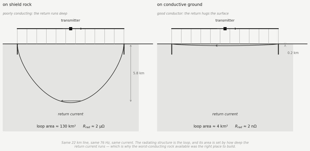
That is the whole antenna. Current leaves the transmitter, travels along the overhead line, enters the earth at one end, returns through the ground, and comes back up at the other. The radiating structure is not the wire. It is the loop — a vertical circuit whose top edge is the line you can see and whose bottom edge is a return path kilometres underground.
Why the ground had to be bad
The two stations sit on the Laurentian Shield, and the sources are explicit that this was the reason for choosing the location: the shield is a very large area of very poor conducting rock.
Read as ordinary engineering that is backwards. Every rule about grounding says to look for conductive, wet, mineral-rich ground, and to avoid dry crystalline rock. Here they went looking for the worst conductor on the continent and built on it deliberately.
The reason is the loop. What radiates is the area the circuit encloses, and that area is set by how deep the return current runs. The governing scale is the skin depth:
which grows as the conductivity falls. In wet, conductive ground at these frequencies the return current hugs the surface, a couple of hundred metres down, and the circuit it closes is a thin ribbon. Under the shield it runs kilometres deep, and the loop becomes a sheet of circuit standing on edge in the crust.
The effective depth is not quite the skin depth of a uniform half-space, because the crust is layered and the current stops where the conductivity rises. The published figures for the two systems make this concrete. Beneath the American antennas the average effective conductivity is about 2.4×10⁻⁴ S/m, giving a working depth near 2.6 km. Under the Kola Peninsula, where ZEVS was built, the first layer is some ten times more resistive still — about 10-5 S/m — and runs about 10 km down before a far more conductive layer stops it. Ten kilometres of usable depth, from ground chosen for being nearly an insulator.
There is a second way to see the same thing. The return current flows opposite to the current in the line, so its field partly cancels the field of the line — this is exactly why a wire lying on a perfect conductor radiates nothing at all. What separates the two currents is depth. Poor conductivity buys separation, and separation is the only thing standing between this antenna and complete self-cancellation.
The numbers, and the other station
The figure of merit ELF designers actually use is not gain or radiation resistance but the magnetic moment of the loop — current, times line length L, times effective depth W:
For the two American antennas together, at 300 A each, 22.5 km long, over 2.6 km of usable depth, that comes to about 3.5×10⁴ A·km².
The Russian station is the useful comparison, because it is the same idea built on different ground. ZEVS sits on the Kola Peninsula near Murmansk: two parallel grounded lines about 60 km long running east–west, driven at 200–300 A, transmitting at 82 Hz. Its moment works out near 1.1×10⁵ A·km² — roughly three times the American figure, which in radiated power is the 10 dB advantage reported when Stanford receivers first picked it up worldwide in January 1990.
Where that advantage comes from is worth reading off the formula. ZEVS runs less current than the American system. It wins on the other two factors: lines nearly three times as long, over ground nearly four times deeper. It is a better antenna mostly because it stands on worse rock.
As for how much actually leaves: a few watts, on both systems. It is worth being careful about where that figure comes from. Treating the circuit as an ordinary small loop radiating into free space,
gives a radiation resistance of order a microohm and, at the documented currents, a couple of tenths of a watt — an order of magnitude below the few watts the operators report. The discrepancy is not arithmetic. A free-space loop formula is the wrong tool here, because the antenna is not radiating into free space: it is launching a mode into the cavity between the ground and the ionosphere, and the coupling to that mode is what sets the output. The free-space estimate is useful for showing the order of magnitude and for comparing one geometry against another; it is not the design calculation.
What is not in doubt is the efficiency. A few watts out of some two and a half megawatts in is under one part per million:
Everything else — better than 99.9999% of the input — warms up Wisconsin, or the Kola Peninsula.
Why that frequency, and what replaced it
Nothing about this design is a free choice. Every feature of it — the hundred kilometres of wire, the megawatts, the deliberate hunt for bad rock — follows from one number, and that number comes from seawater.
Salt water is a conductor, and a conductor screens. A signal entering the ocean dies away over the same skin depth of Formula 1, now with the conductivity of seawater, about 4 S/m. In the VLF band around 20 kHz that distance is under two metres: a boat has to come to periscope depth and put an antenna near the surface, which is exactly what a submarine exists not to do. At 76 Hz it is about twenty-nine metres, and the boat can stay deep and fast. That single factor of sixteen is the entire justification for the enterprise.
Which is also why the whole system is built around the magnetic field and never the electric one. Seawater does not merely attenuate an electric field, it shorts it out: the free charges rearrange and cancel it, in the way any conductor does. The magnetic field is attenuated, by the skin depth above, but it is not suppressed by that mechanism, and it survives. So the receivers are magnetometers — ferromagnetic-cored solenoids on a trailed antenna in the ordinary case, and triaxial SQUID arrays, specified at around ten femtotesla per root hertz, in the version built for the deepest and fastest boats. That closes the circle back to the transmitter: the design figure at one end is a magnetic moment, and the sensor at the other end measures a magnetic field. The electric field never enters the useful account at either end.
The amplitudes involved are worth stating, because they are the other half of why the bandwidth is what it is. A field of order a picotesla at the surface, attenuated through a hundred metres of seawater, arrives at the boat as a few tens of femtotesla — something like a billionth of the Earth’s own steady field, in which the sensor is sitting, and below the natural background of lightning and Schumann resonance in the same band. Pulling a signal out of that takes a very narrow bandwidth and a long integration, which is another way of saying: a few characters per minute.
The bill for it is bandwidth. At these frequencies there is essentially none: the system sent short coded messages at a few characters per minute, one way, with no possibility of a reply — the transmitter needed a hundred kilometres of antenna, and no submarine carries one. In practice it was a bell rather than a telephone: a signal telling a boat to come shallow and listen properly on a faster channel.
Which is, in the end, how it was superseded. Project ELF was shut down in September 2004, declared obsolete in favour of improved VLF systems. The replacement does not solve the seawater problem — nothing solves the seawater problem — it goes around it by moving the receiver instead of the signal: towed buoys and trailing wire antennas that a submarine streams close enough to the surface to use ordinary VLF, while the hull stays deep. That is better engineering, and it also concedes the point the ELF system had been built to avoid. Something has to come up. For fifteen years, nothing did.
ZEVS, by the available accounts, is still there.
An echo
One detail is hard to pass over. The final grounding arrangement at these stations was arrays of electrodes in boreholes 300 feet deep.
Three hundred feet of iron pipe driven into bedrock is also, to the foot, what Tesla had sunk beneath Wardenclyffe eighty years earlier, and for the same stated reason: to get a grip on the earth. Two projects with almost nothing else in common — one a private venture built on a misconception, the other a cold-war military system built on correct theory — arrived at the same answer to the same narrow question of how to put current into the ground.
They diverge immediately afterwards, and the divergence is the whole difference between them. Tesla ran his conductor up, into a single elevated terminal, and expected the Earth to carry the energy onward by conduction. These stations run their conductor sideways, twenty kilometres to a second ground point, and expect nothing of the Earth except that it close a circuit and stay out of the way. What radiates is the loop; what carries the signal is the waveguide between the ground and the ionosphere, with the energy travelling in the air above the surface rather than in the rock below it.
Same band, same grounding problem, same solution to it — and opposite conclusions about what the planet is for.
Sources
Project Sanguine and Project ELF: transmitter geometry at Clam Lake, Wisconsin and Republic, Michigan; 84 miles of above-ground line; grounding by buried cable and by electrode arrays in 300 ft boreholes; the 1968 proposal for a 6,000-mile buried grid over 22,500 square miles.
U.S. Navy operational descriptions of the ELF system, 76 Hz, one-way messaging to submerged submarines; Clam Lake trials of 1983–84 (communication with a boat at 400 ft and 16 knots); shutdown in September 2004.
ZEVS, Kola Peninsula: two parallel grounded lines about 60 km long, east–west, 82 Hz, 200–300 A. E. P. Velikhov et al., 1996 and 1998; A. C. Fraser-Smith, “Reception of ELF signals at antipodal distances” (Stanford), on the worldwide reception of the 82 Hz transmissions in January 1990 and the 10 dB advantage over the American system.
Ground conductivity and effective depth figures for both sites (2.4×10⁻⁴ S/m and W ≈ 2.6 km beneath the American antennas; a resistive first layer of about 10-5 S/m to some 10 km depth under the Kola Peninsula), and the magnetic-moment comparison, from the technical summaries at vlf.it.
Michigan Technological University, Military History of the Upper Great Lakes, student research pages on the Clam Lake and Republic installations (source for the input power, the radiated power, and the choice of the Laurentian Shield for its low conductivity).
Submarine ELF reception: development of triaxial SQUID receiving antennas with sensitivity of order 10-14 T·Hz-1/2, and detection of the Wisconsin transmitter at 100 m depth (IEEE literature on superconducting ELF magnetic field sensors).
Radiation resistance of an electrically small loop: standard antenna theory, e.g. C. A. Balanis, Antenna Theory: Analysis and Design.
Skin depth and seawater attenuation: J. D. Jackson, Classical Electrodynamics, 3rd ed., ch. 5 and 7.
Wardenclyffe grounding: L. I. Anderson (ed.), Nikola Tesla On His Work With Alternating Currents, 1916 deposition; discussed at length in The Antenna That Wasn’t One on this site.
In 1901, on two hundred acres of Long Island scrubland, Nikola Tesla began building the first station of what he called the World Wireless System. A friend recalled him speaking of more than thirty transmitting and receiving stations at the world’s major population centres, though that figure comes from the secondhand account rather than from anything Tesla published; what is documented is that Shoreham was to be followed by a plant in the British Isles, possibly on the west coast of Scotland. Each station was to send and receive both signals and usable electrical power, without wires. The 187-foot structure at Shoreham, topped by a dome roughly sixty-eight feet across, was funded by J. P. Morgan with $150,000 — real money, from the most powerful financier in America. By around 1906 work had effectively stopped, on the sole station of the network ever begun, though Tesla stated in his 1916 deposition that he had continued using the antenna until 1907. In 1917 it was demolished for scrap.
The standard telling treats this as a story about money: a genius undone by a financier who got cold feet. That part is true as far as it goes. The standard technical telling treats the tower as a radio antenna that was never going to broadcast power around the planet, and that part is also true — but it rests on reading the tower as something Tesla’s own writing never quite calls it. Read literally, what he describes is a machine with two distinct jobs, only one of which is radio at all. Untangling the two turns out to matter a great deal for what the numbers say.
What Tesla said the tower would do
Tesla was explicit about the mechanism, not just the goal. Writing in Collier’s Weekly in February 1901, he described a system using “the Earth itself as the medium for conducting the currents, thus dispensing with wires and all other artificial conductors” — a transmitter that would act “like a pump,” drawing electricity from the Earth and driving it back in, producing disturbances that would spread through the Earth as through a wire, detectable at any distance by a properly tuned receiver. “It is necessary for the machine to get a grip of the earth,” he said of the underground works beneath the tower, “so that the whole of this globe can quiver.”
He was equally explicit about the efficiency, though the claim comes much later than the work. Describing the 1899 Colorado Springs tests he took as proof of concept, he would write that he had found the current “capable of passing across the entire globe and returning from the antipodes to its origin with undiminished strength,” and that power could be conveyed “at any distance, limited only by the physical dimensions of the globe, with an efficiency as high as ninety-nine and one-half per cent.”
That figure, 99.5%, is the claim this article tests — but its provenance deserves stating, because it is not what it is usually taken to be. The passage appears in “World System of Wireless Transmission of Energy,” published in Telegraph and Telephone Age on 16 October 1927: twenty-eight years after the experiments it describes, and a decade after the tower had been demolished for scrap. It is a memoir, not a design specification, and nothing was built to it.
The same sentence carries a figure worth pausing on. Tesla states that he ran those Colorado Springs tests “with a generator of fifteen hundred kilowatt capacity.” The transformer documented in his own notebooks was rated around 50 kVA. The two numbers need not contradict each other: his power came from the El Paso Electric Company, and 1,500 kW plausibly describes the capacity of the city plant supplying him rather than what his apparatus drew. Read that way the sentence is literally true and measures a different thing.
But the context is a description of the scale of his own experiments, and a reader who takes the figure as offered will come away with an impression the notebooks do not support. Whichever reading is right, the efficiency claim remains worth testing — it is precise enough to be falsified, which is more than most such assertions manage. It should simply be read for what it is: a recollection set down decades after the fact, in a text where at least one number invites a more generous impression than the record gives.
The word doing the work in the first quotation is conducting. Not one time, in passing, but repeatedly and as the organising idea of the whole system: a closed electrical circuit, the tower and the distant Earth as its two terminals, through which power flows the way current flows through a wire.
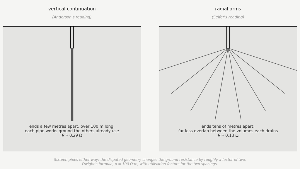
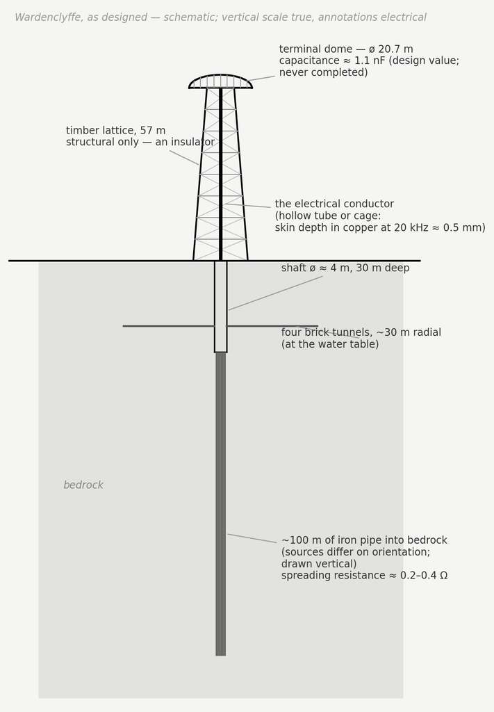
He took the resistance side of that picture seriously, and it is worth saying so plainly before anything else, because the usual telling does not. Beneath the tower he sank a shaft some 120 feet into the ground, and from its bottom had roughly 300 feet of iron pipe driven onward into the bedrock, using machinery built for the purpose. Sources disagree about the orientation: Anderson reads the pipes as continuing vertically, to some 420 feet in total, while Seifer describes sixteen radial arms spreading outward from the central shaft. What is not in dispute is a set of four brick-lined tunnels, each about a hundred feet long, running radially outward at the water table.
The disagreement does not matter for the argument here, which is why it can be stated plainly rather than resolved. On either reading this was a grounding system of unprecedented scale for a private laboratory, and on either reading it is what one builds for a machine intended to drive current into the ground rather than to radiate into the air.
It does change the numbers, though, and by more than one might expect. Note first what Anderson’s reading actually claims: not sixteen separate electrodes, but a single pipe made of sixteen lengths joined end to end — the deposition’s “one length after another” — driven straight down. At 300 feet in sixteen sections that is about nineteen feet per length, an entirely ordinary size of pipe section. On that reading there is one electrode, not sixteen.
The difference matters because the resistance of a ground system depends on the extent of soil it reaches, not on how much iron it contains. A single deep pipe, however long, drains one narrow column: Dwight’s formula gives roughly 1.2 Ω. A radial fan behaves quite differently, and not for the reason one might guess — the arms are not independent electrodes, since near the hub they are centimetres apart and their fields overlap completely. What the array does is act as a disc electrode whose radius is the arm length, and the resistance of a disc falls as the inverse of its radius. For arms of this length that gives roughly 0.15–0.27 Ω, close to an order of magnitude better, with the same total iron in the ground.
One consequence worth noting is that sixteen arms are well past the point of diminishing returns: eight would give nearly the same result, since what counts is the radius reached, not the number of spokes.
That is an argument on engineering grounds rather than documentary ones, and it is worth flagging as such. But a factor of ten is not a subtlety, and a designer who had already paid to drill and drive 300 feet of pipe would have gained enormously by fanning it out rather than sinking it in a single line. The sources remain where they are; if one had to guess which arrangement a careful engineer would have chosen, the numbers point one way.
Two jobs, easily read as one
It would be a mistake to read Tesla’s conduction language as the naivety of someone unfamiliar with radio. He was, if anything, the opposite: the U.S. Supreme Court’s 1943 ruling in Marconi Wireless Telegraph Co. v. United States invalidated Marconi’s core tuning patent partly on the grounds that Tesla’s own prior patents had already disclosed the same tuned-circuit principles Marconi later claimed. Whatever else is true about the messy question of who invented radio, Tesla’s command of resonant RF circuits was real, well ahead of most of his contemporaries, and legally recognised as such.
That competence shows directly in the transmitter’s design. The resonant coil driving the elevated terminal — the “extra coil” of Tesla’s magnifying transmitter — was wound to present an electrical length near a quarter wavelength. That is the standard technique for building up a large voltage at an open, high-impedance end from a modest voltage at the driven end. The Wardenclyffe coil used the same architecture as the one at Colorado Springs but, on the available evidence, a markedly different shape: Anderson reads the drawings in patent 1,119,732 as giving a height-to-diameter ratio around 9:1, against roughly 1:1 in Colorado. Those drawings come from the patent’s 1907 renewal, however, and may reflect a later design rather than what was actually erected at Shoreham between 1901 and 1903. This is correct, sophisticated radio-frequency engineering, and it solves a specific problem: how to charge an elevated terminal to millions of volts efficiently. It says nothing, by itself, about how power gets from one station to another once that terminal is charged.
Here is the conflation worth naming directly: reading a resonant coil charging an elevated capacitive terminal, one reaches automatically for the vocabulary of radio — wavelength, radiation resistance, antenna gain — because that vocabulary is built for exactly this kind of hardware. But Tesla’s own words assign the apparatus two distinct jobs at a single frequency. The resonant stage multiplies voltage locally, so that charge can be driven into the ground at each station; the job of moving that energy from station to station is assigned, in his writing, to the Earth itself as a conductor. One frequency, two functions — and the two functions turn out to behave very differently when each is tested on its own terms.
The geometry of the local apparatus
Electrically, the tower and its terminal dome form what antenna theory calls a top-loaded monopole: a vertical conductor topped by a large capacitive terminal (the dome), standing on a conducting ground plane (the Earth). The wooden lattice visible in photographs of Wardenclyffe was structural, not electrical — wood is an insulator — so the actual current-carrying path was a separate conductor, almost certainly a copper cable, run up through or alongside the wooden framework to the dome. This was standard practice for the period: low-frequency stations of that era, including Marconi’s, routinely supported their electrical conductors on wooden or lattice-steel masts that carried no current themselves. Electrically, what matters is the height the conductor spans and its own capacitance, not the material of whatever holds it up. Tower conductor and dome are the same electrical node — wired together, they rise and fall in potential as one — so their capacitances to ground simply add:
For the dome, approximated as an isolated sphere of radius a ≈ 10.3 m, the capacitance works out to about 1.1 nF — matching, reassuringly, the roughly 1 nF Tesla himself specified as a design target for the terminal. Design target is the right phrase: the dome was never finished. Photographs show partial ribbing and no completed surface, sources disagree on how far the work got, and every capacitance figure in this article is therefore computed from the intended geometry rather than measured on a built structure. The conductor’s own contribution is harder to pin down precisely, since its exact diameter is not documented in the sources consulted for this article. Fortunately the formula for a thin conductor’s capacitance depends on its radius only logarithmically, so the uncertainty barely matters: plausible radii from 1 to 20 cm all give roughly 380–590 pF. The larger end of that range would not have been a solid cable — at that thickness it would necessarily have been a hollow tube or a cage of several thinner conductors bundled to present a large effective radius. Two independent reasons favour this over solid metal, and the more fundamental of the two is skin effect. At 20 kHz, alternating current in a conductor is confined to a thin layer near its surface; in copper the skin depth at that frequency is only about 0.5 mm, so a solid rod of any real thickness would carry its current in a shell under a millimetre deep, with everything beneath it electrically inert. A hollow tube of the same outer radius carries essentially the same current at a fraction of the weight and cost — which is also, independently, the standard period technique for suppressing corona without the weight of solid metal, and the same principle behind the dome itself, which was a shell rather than a solid sphere. Either way the dome dominates, but the conductor’s own contribution is not negligible.
The dome’s real job, though, is not capacitance for its own sake. A bare vertical wire above a ground plane carries current that tapers to zero at its open top — there is nowhere left for the charge to go — which halves its effective radiating height compared to its physical height. A large capacitive top load gives that current somewhere to flow into instead of dying away, keeping it closer to uniform along the whole structure. This is the actual engineering reason for building a wide top-hat structure at all, and it is worth being precise about which of the tower’s two jobs it serves: it does help the antenna-reading of the structure, discussed next, but its more direct purpose in Tesla’s own account is charging the terminal to the voltage needed to drive current into the ground.
Testing the antenna reading first
Before turning to the conduction picture Tesla actually describes, it is worth finishing the antenna calculation this site’s earlier draft of this article was built around — because it is the reading almost every account of Wardenclyffe reaches for by default, and because knowing precisely how it fails is what makes the alternative worth taking seriously.
A vertical monopole of height h standing on a perfectly conducting ground plane produces, in the space above the plane, exactly the field of a full dipole of height 2h in free space — the missing lower half supplied by its mirror image in the conductor. For Wardenclyffe: a 57 m tower behaves, above ground, like half of a 114 m dipole.
Two corrections keep this equivalence from being used carelessly. First, the real structure only radiates into the half-space above ground, which by itself halves the radiation resistance relative to the naive free-space dipole formula. Second, the equivalence assumes a perfectly conducting ground plane, which the sandy soil of Shoreham was not.
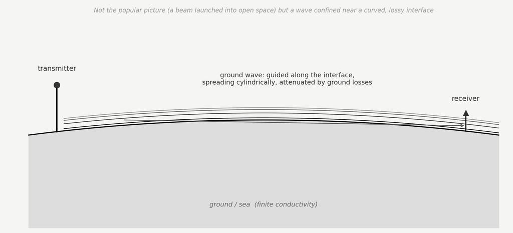
The intuitive picture of what happens next — a beam launched into open space, the way a searchlight throws a beam — is not the geometry a ground-based low-frequency transmitter produces, and if the goal really were direct station-to-station radio transmission it would need to be a ground wave: a disturbance bound to the interface between the (poorly) conducting Earth and the air above it, spreading cylindrically rather than spherically, but continuously bleeding energy into the ground it rides along.
None of that matters, however, until a more basic question is settled: how much of the power fed into the tower becomes a travelling wave at all, as opposed to heat. For a top-loaded monopole with a genuinely uniform current, image theory gives the radiation resistance over an ideal ground plane as:
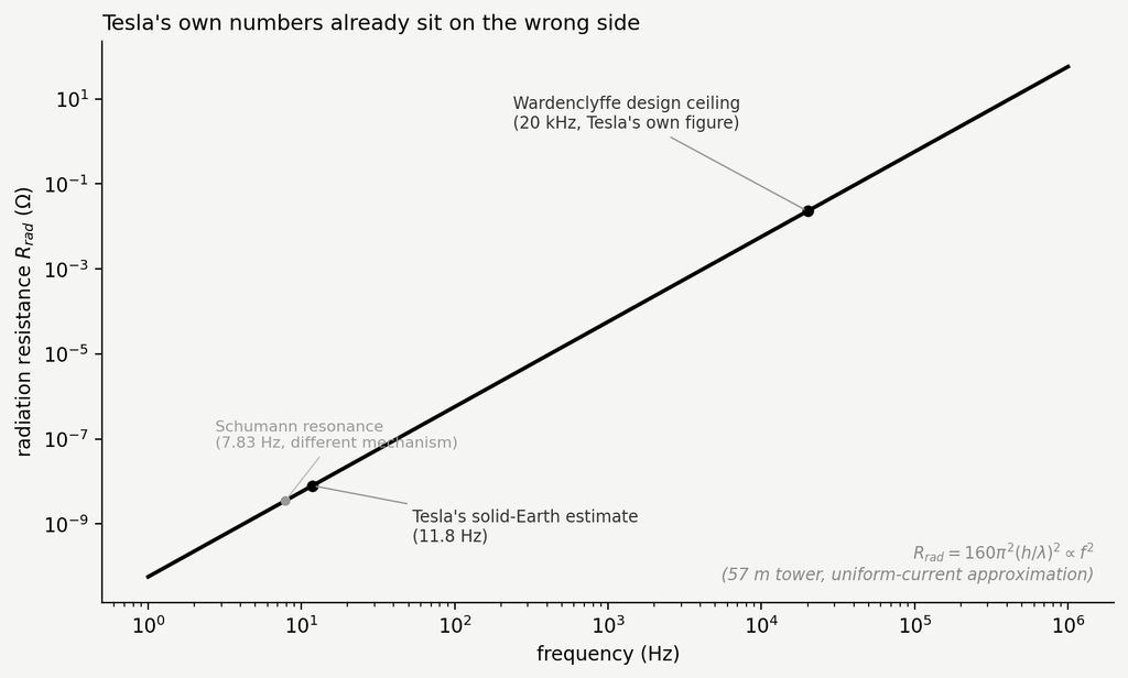
Putting in the real numbers — h = 57 m, and an operating frequency of 20 kHz, the upper bound Tesla himself specifies (his stated reason for it is examined further below) — gives a wavelength of about 15 km and a radiation resistance of:
A few hundredths of an ohm. Whatever fraction of the fed-in power actually leaves as a travelling wave is set by how this tiny resistance compares with everything else in the circuit that also consumes power:
Ground resistances for radiating structures of this kind typically run from several ohms to several tens of ohms. At 5 Ω the radiating efficiency is under half a percent; at 25 Ω, about one part in a thousand. Those typical figures are worth reading carefully: they describe stations that already have a radial ground mat installed. A tower without one does worse, not better, so for Wardenclyffe these numbers are if anything optimistic and the half-percent should be read as an upper bound.
These figures also need a word of explanation, because a later section of this article puts the ground system Tesla actually built well below one ohm. The two sets of numbers are not in conflict and cannot be compared directly, because they are not the same physical quantity — and understanding why turns out to be one of the sharpest pieces of evidence in the whole case.
The spreading resistance computed later is a direct-current quantity: the resistance from an electrode to remote earth, dominated by the material in the electrode’s immediate vicinity, and therefore improved by driving deep into conductive rock. The loss resistance that matters to a radiating monopole is something else entirely. The antenna’s return currents flow through the soil across the whole region within roughly a quarter wavelength of the base — at 20 kHz, a disc some 3.75 km in radius — and it is dissipation in that vast shallow area, not at the electrode, that consumes the power. A deep shaft does essentially nothing for it. This is precisely why real low-frequency broadcast stations do not sink shafts: they lay out radial wire mats spreading kilometres from the tower base, buried just below the surface, to intercept those return currents before they dissipate in the ground.
Tesla built the shaft. He did not build the radial mat. His grounding system was optimised, at considerable expense, for exactly the quantity that matters to a conduction machine and is nearly irrelevant to a radiating one — which is a stronger argument about what he thought he was building than anything in the written record.
Taken purely as an antenna, then, the verdict is not close. A fraction of a percent against a claimed 99.5% is not a shortfall to be closed with better engineering, and no choice of frequency rescues it: pushing lower to improve the geometric spreading only crushes the radiation resistance further, since it scales as the square of frequency. Nor does moving within the band Tesla himself specifies help — at the 5.9 Hz bottom end of his stated range, the radiation resistance of a 57 m tower falls by another seven orders of magnitude from the already-poor 20 kHz figure, to a couple of nanohms. There is no frequency, anywhere in his own window, at which this structure is a viable radio transmitter for the distances involved.
Taking the conduction language literally
This is the point at which Tesla’s own words stop fitting the antenna reading at all. He never describes station-to-station radio transmission as the long-range mechanism. He describes current entering the Earth at one station and reappearing at another, having travelled through the planet rather than around it or above it. Taken literally, this proposes a machine whose two jobs are not both radio: a resonant stage (the extra coil) that charges the elevated terminal to a high voltage, and a conduction stage that carries current between stations through the body of the Earth once that charge is dumped to ground. The frequency at which the second stage operates is not something to be guessed at — Tesla specifies it, along with two other conditions, in a patent examined below.
On this reading, the radiation-resistance collapse calculated above is not a fatal flaw. It is irrelevant, because the RF stage was never meant to radiate the intercontinental link in the first place — its job ends once it has raised the terminal to the design voltage. The question worth asking is not whether the tower radiates efficiently over thousands of kilometres. It is whether current at the frequencies Tesla specifies conducts efficiently through the Earth over that range, which is an entirely different calculation.
One clarification belongs here, because the alternative circulates widely. Many accounts of Wardenclyffe describe a two-legged circuit: current out through the ground, and back through a conducting layer in the upper atmosphere. Carlson’s biography describes the return path that way, and popular summaries go further, adding an ultraviolet beam to ionise a conduction channel deliberately.
Tesla did patent that scheme — but earlier, and it does not govern the tower. Two applications filed on the same day, 2 September 1897, cover it: U.S. 645,576 and U.S. 649,621, the first explicitly allowing the lower atmospheric strata as a conducting path, with a demonstration before the Patent Office in January 1898 showing transmission through a rarefied medium with ground return. That work predates Colorado Springs. What came after it, in the patent filed in May 1900 and covering the system Wardenclyffe was built to embody, is the passage quoted earlier: the planet behaving as a perfectly smooth conductor of inappreciable resistance, with capacitance and self-induction distributed along the axis of propagation. As Jackson notes in discussing that text, Tesla is treating the Earth as a perfectly conducting sphere in infinite space — and a sphere in infinite space has no second plate and no return path. The atmosphere is simply absent from the model.
It could hardly have been otherwise. The conducting layer that would later make sense of a two-legged circuit was not a known object in 1900: Kennelly and Heaviside proposed it independently in 1902, and it was confirmed only in 1924–25. What Tesla had was the general notion of conducting air strata somewhere high up, and his own estimate that reaching them would need an antenna some twenty-five kilometres tall. The tower is 57 metres. Whatever the 1897 patents envisage, Wardenclyffe was built for the single-path system, and that is the one tested here.
The local leg: injecting current into the ground
For a compact electrode driven into a much larger conducting medium, the resistance to remote earth is dominated by the material in the immediate vicinity of the electrode — a classical result, the same mathematics that makes the capacitance of an isolated sphere independent of where a distant return path happens to sit. The standard engineering formula for a vertical driven rod of length L and radius a, in soil of resistivity ρ, is:
Applied to roughly 100 m of iron pipe in moderately conductive rock, a single deep electrode gives about 1.2 Ω. If the iron was instead fanned out radially, as Seifer reads it, the array behaves as a disc electrode of radius equal to the arm length, and the figure falls to somewhere between 0.15 and 0.27 Ω depending on how deeply the disc sits. The honest range across both readings is therefore roughly 0.15–1.2 Ω — and the conclusion does not depend on which end of it is right.
What matters is the asymmetry, not the number. On either reading this was an excellent ground connection by the measure that governs conduction into the earth. And on either reading it did nothing whatever for the loss that governs radiation, which is dominated by dissipation across kilometres of shallow soil that no electrode, however deep, ever touches. One structure, excellent by one measure and simply irrelevant to the other: that is what discriminates between the two readings of the tower. This reframes a piece of the design that looked eccentric under the antenna reading: an ordinary radio antenna reduces ground loss with a field of shallow surface radials, not pipes driven a hundred metres into bedrock. Driving deep only makes sense as an attempt to punch through a resistive near-surface layer into more conductive material below — which is precisely what a conduction-based system, not a radiating one, would need.
The global leg: how far does the carrier actually reach
The local result is encouraging. Whether the same current can then travel usefully between continents is a separate question, and the answer is less settled — but it has to be asked at the right frequency. As the next section works through in detail, the frequency Tesla specifies for the propagating carrier is not the often-quoted 11.8; it is a band running from about 5.9 Hz at the bottom to a stated ceiling of 20 kHz at the top. The question is what happens across that band.
A first check is whether the planet is even electrically “small” at these frequencies, the condition under which a circuit description makes sense at all in place of a radiating one. It depends sharply on where in the band one sits. At the 5.9 Hz bottom end, the free-space wavelength is about 51,000 km — longer than the Earth’s circumference, though only by a factor of 1.3, which is marginal for a lumped-element description rather than comfortably within its domain. At the 20 kHz ceiling it is 15 km, thousands of times smaller than the Earth, and no such description applies. Tesla’s own stated band spans both regimes.
Consistency is not sufficiency in either case, though. An oscillating current does not travel through a lossy conductor unattenuated; it diffuses, penetrating to a characteristic skin depth that shrinks as either frequency or conductivity rises:
Evaluated across Tesla’s band in moderately conductive, water-saturated crustal rock, the penetration depth runs from roughly two kilometres at 5.9 Hz down to a few tens of metres at 20 kHz. Even the most favourable case is a small fraction of the Earth’s radius, and in most cases a small fraction of the crust’s own thickness. The current does not reach the far more conductive mantle. It stays confined to a shallow shell near the surface, and must cross intercontinental distances within that shell rather than through the planet’s bulk — and the higher in his own band the system is tuned, the thinner that shell becomes.
And here the two readings this article has been keeping apart collapse into one. A disturbance confined to a shallow shell at a conducting interface, spreading cylindrically and bleeding energy into the lossy medium as it goes, is the ground wave — the same object worked through for the radio-frequency case above, in a different vocabulary. Crustal conduction and Norton’s ground-wave propagation are not two competing mechanisms between which Tesla’s design must choose. They are the same phenomenon described twice, and the attenuation calculation for it was published by Norton in 1936.
Crustal conductivity does vary by orders of magnitude with local geology — sedimentary basins against crystalline shield rock, continental crust against ocean floor — and that variation is real. But it changes the value, not the order of magnitude of the comparison, and the comparison is not favourable: a channel confined within kilometres of lossy rock is far more dissipative than one propagating above the surface.
One general point does survive the uncertainty, and it favours a choice Tesla made anyway. Resistance per unit length along the shallow conducting shell scales as the inverse square root of the material’s conductivity, since higher conductivity lowers the resistivity and compresses the current into a thinner skin at the same time. Seawater, at roughly 4 S/m, is some four hundred times more conductive than the wet sedimentary rock assumed above — which, after the square-root scaling, still leaves an oceanic path about twenty times less resistive per unit length than a continental one. Good grounding practice had favoured wet, conductive ground over dry rock long before anyone could calculate a skin depth, and Wardenclyffe sits on a coastal site, as did most of the locations associated with Tesla’s later station proposals. The choice was very likely made for ordinary electrical reasons. It happens also to be the right one for the reason worked out here.
Tesla’s own three requirements
The two-stage picture above raises an obvious question: if a radio-frequency stage charges the terminal and a conduction stage carries the energy between stations, at what frequency does the second stage actually operate? It is tempting to answer by inventing a mechanism — a low-frequency envelope on the carrier, say, demodulated by the ground itself. Tesla’s own patent makes such invention unnecessary, and shows it to be wrong.
In U.S. Patent 787,412, Art of Transmitting Electrical Energy Through the Natural Mediums — filed May 1900, renewed June 1902, granted April 1905 — Tesla sets out three conditions he considers essential for establishing the resonant state. (They reached the file late, as the last part of this section shows; but they are the fullest statement he left of what the system needed.) They are worth taking one at a time, because they do not all constrain the same quantity, and the most-quoted number among them turns out not to be a frequency at all.
The first is geometric, and it constrains the carrier. Tesla requires that the Earth’s polar diameter be an odd multiple of a quarter wavelength — that is, of the ratio between the speed of light and four times the frequency of the currents. Worked through, 12,742 km set equal to c/4f gives a fundamental near 5.9 Hz, which matches the “six per second” he cites shortly afterwards. The odd-harmonic criterion so often attributed to Tesla originates here, and it applies to the carrier.
The second sets bounds on that same carrier. Tesla specifies that the frequency should be below 20,000 per second, with a minimum around six per second, below which — as he explains — the Earth ceases to resonate at all and behaves simply as a capacitance whose potential varies almost uniformly over its whole surface. The upper bound is worth reading carefully, because his stated reason for it is not the one this article assumed earlier: in the patent, the 20 kHz ceiling is justified by the need for oscillations whose rate of radiation into space in the form of Hertzian waves is very small — suppressing radiation, not minimising ground-wave attenuation. The attenuation reading comes from the Colorado Springs Notes and from later commentators. Two distinct criteria, arriving at the same order of magnitude for different reasons.
The third is the one that is almost universally misread, and Tesla states it with unusual precision. The most essential requirement, he writes, is that — irrespective of frequency — the wave or wave-train should continue for a certain interval of time, which he estimates at not less than about 0.08484 s: the time taken to travel to the region diametrically opposite the pole and back, at a mean surface propagation velocity of roughly 471,240 km/s.
Those two words, irrespective of frequency, do a great deal of work. The 0.08484 s figure is not a resonance, not an envelope, and not a spectral line. It is a minimum duration for each wave-train — a coherence requirement. Its operational consequence is a limit on how fast the system can be keyed: if every train must last at least 0.0848 s, the maximum signalling rate is about 11.8 symbols per second. That is a baud rate, not a frequency to be generated.
This matters because 11.8 is the number that most often escapes into secondary accounts as though it were a resonance of the Earth, and it is not. Nor is it the same quantity as the 5.9 Hz of the first requirement, despite the tidy factor of two: 5.9 Hz derives from the Earth’s diameter, while 11.8 per second derives from its circumference — 40,000 km divided by 471,240 km/s. Different geometry, different physical quantity, related by coincidence of arithmetic rather than by physics. (The velocity itself is not measured but derived: 471,240 km/s is (π/2)·c to three figures, a consequence of the surface-propagation model Tesla develops in the Colorado Springs notebooks.)
What Tesla did and did not propose about two wavelengths
Emitting more than one wavelength at once is Tesla’s own idea, and it is in the patent: he describes impressing upon the Earth two or more oscillations of different wavelength so that a resultant stationary wave travels slowly over the globe, and claims 5 and 6 cover varying the wavelengths and shifting the nodal and ventral regions respectively.
But the stated purpose is not to synthesise a low-frequency envelope. It is to make the standing-wave pattern migrate across the Earth’s surface, so that a maximum can be brought to coincide on command with a chosen receiving station. This is addressing and scanning, not coupling to a terrestrial resonance. The same reading applies to his manuscript note of 2 June 1901 on spatially modulated wave groups: concentrating energy into concentric rings, not building an ELF component.
Synchronisation to a pulse train does appear in the patent — but at the receiver, not the transmitter. Tesla describes a rotating insulating cylinder carrying metallic segments that accumulate the energy of an arbitrary number of successive impulses onto a condenser, which a second segmented cylinder then discharges into the receiver at predetermined intervals. It is a synchronous integrator, effectively coherent detection avant la lettre, and its purpose is sensitivity on weak signals. It has nothing to do with generating a low-frequency component at the transmitting end.
The distinction is worth stating plainly because the alternative reading is widespread: the interpretation of Wardenclyffe as broadcasting an ELF signal superimposed on an HF carrier belongs to K. L. and J. F. Corum, in work presented at the 1996 International Tesla Symposium, and is explicitly offered there as a reconstruction rather than as a reading of the text. Tesla’s third requirement makes such a mechanism unnecessary on his own terms: his 0.0848 s constraint is about duration, not spectrum, and nothing in the patent asks the transmitter to produce a second frequency at all.
The requirements do not fit together
Taken as a set, the three conditions are in tension, and the tension is quantifiable.
The first requirement admits any odd multiple of about 5.9 Hz; the second caps the carrier at 20 kHz. Some 1,700 admissible odd harmonics fall inside that window, spaced 11.8 Hz apart. At the top of the range this means a fractional spacing of roughly 6×10⁻⁴ — so distinguishing one admissible harmonic from its neighbour would demand a Q of order 1,700 across the entire system, Earth included. No spark-gap transmitter, however well quenched, approaches that. The first requirement is therefore very nearly non-binding in the upper part of the band Tesla himself specifies: almost any tuning falls close enough to some odd harmonic to satisfy it formally. It has real force only near the bottom, where the admissible harmonics are sparse.
This was not missed at the time. In the official action of 24 September 1903 on the application (Serial No. 112,034), the examiner observes that, given what Tesla states in the second requirement — a ventral region opposite the source and a node at the ground plate — it should be the Earth’s semi-circumference, not its diameter, that must be an odd multiple of the quarter wavelength.
The objection is more than procedural, and the physics behind it is worth spelling out, because it is the same point arrived at from a different direction. Inside a conductor, electromagnetic fields do not propagate as waves at all — they diffuse, governed by a parabolic equation rather than a hyperbolic one, on timescales set by conductivity and the square of distance rather than by any velocity. For the Earth as a whole those diffusion times run to millennia, which is why the geomagnetic field changes on geological timescales and why the geodynamo has to be explained by convective motion rather than passive field diffusion. Nothing at Tesla’s frequencies penetrates more than a few kilometres into the crust, as the skin-depth figures above already showed. A path through the Earth, along its diameter, is therefore not available to the signal at all. Whatever travels between two stations travels along the surface, and the geometrically relevant distance is an arc, not a chord.
Tesla knew this at some level, because his own third requirement uses the circumference: the 0.08484 s figure is a round trip along the surface. Yet his first requirement uses the diameter. The two cannot both describe the same signal.
There is a curious resolution buried in the numbers, and it turns on a factor of π. The Earth’s semi-circumference is π/2 times its diameter. And Tesla’s surface propagation velocity, 471,240 km/s, is π/2 times the speed of light to three figures — exactly the factor needed to make a diameter-based formula return the same answer as a semi-circumference-based one. Worked through: the quarter-wave condition on the polar diameter, evaluated at c, gives 5.88 Hz. The same condition on the semi-circumference, evaluated at Tesla’s own velocity, gives 5.89 Hz. The two π/2 factors cancel, and the fundamental frequency comes out identical either way.
None of which is a modern observation. The examiner had already made it, in the same 1903 action, and set it down in a single sentence: the applicant’s value of v is 1.57 times the value hitherto established, and that factor is the ratio of semi-circumference to diameter. He then draws the consequence with some care — if the applicant’s velocity is correct, there is no discrepancy between the first and third requirements at all.
And then he closes the trap. That velocity is not offered in the patent as a special surface-propagation figure, distinct from the speed of light and legitimately different from it. It is offered as the value of v, the same quantity everyone else had measured. So making the requirements consistent means asserting that v is half again as large as the figure “determined by Maxwell, Rowland, Hertz and many other distinguished physicists, such as Weber & Kohlrausch, Ayrton & Perry and Kelvin” — and the examiner, listing them by name, observes drily that such a startling discovery would need to be rigorously substantiated.
That disposes of the charitable reading. The π/2 factor is not a geometric conversion openly declared; it is a claim about the speed of light, made in order to reconcile two requirements that would otherwise contradict each other. It is one thing to write a condition in terms of the diameter while knowing the path is an arc. It is another to keep the diameter and adjust the speed of light to suit.
The same document settles a question of chronology, in a line easy to pass over: none of the three essential requirements were in the application as originally filed. They entered in an amendment of August 1903 — three years after the filing date, four years after Colorado Springs, and two years into construction at Shoreham. They are not the design criteria the tower was built to. They are theory written afterwards, to account for a structure that was already standing, and they arrived a month before an examiner took them apart.
His proposed remedy is worth quoting for what it says about the state of the argument: the best way out of the difficulty, he wrote, would be to cancel all reference to the first and third, and possibly the second, essential requirements, and submit a showing of operativeness together with the constants of the apparatus as a substitute for theory.
It is a small episode, and an unusually clarifying one. The system’s own designer had specified three conditions that could not all be satisfied as stated; the first person on record to notice was not a physicist but the examiner whose job was to read the claims carefully; and his advice, in the end, was to stop explaining and start demonstrating.
There is a second gap of the same kind, this one between what Tesla prescribed and what he built. The patent caps the carrier at 20 kHz. The extra coil he actually constructed and measured at Colorado Springs self-resonated at 86.8 kHz, and around 48 kHz once loaded by the antenna’s own capacitance — in both cases well above his own stated ceiling. The hardware he had in hand, and whose resonance he recorded in his notebooks, did not satisfy the requirement he was setting out in the patent he filed at the same time — the application went in on 16 May 1900, while the Colorado Springs work was still under way. He was prescribing the ceiling while the apparatus that exceeded it stood running in front of him.
What the two-function reading changes
It changes the verdict on Tesla’s engineering without rescuing the system. Read as a single radio antenna, Wardenclyffe fails by many orders of magnitude at every frequency in Tesla’s own stated band, and several of its design choices — the extreme depth of the ground system above all — look like overkill or confusion. Read as his own words describe it, one frequency serving two functions, the resonant engineering is sound and well within his demonstrated competence, and the deep grounding is exactly the right response to the problem it was actually solving: not reducing loss in an antenna, but establishing a low-resistance path for current into the Earth.
What that reading does not do is make the long-range half work. The local numbers are good. The global ones run into the medium: a current confined to a shallow shell of lossy rock, asked to cross intercontinental distances within it, is a ground wave by another name — and one routed through the most dissipative path available. Long-range propagation at these frequencies is entirely real, as VLF navigation and communication systems demonstrated for decades. It just does not happen in the rock.
What was salvageable, and what remains open
The Earth and the ionosphere really do form a resonant electromagnetic cavity, and it really does support standing-wave resonances at extremely low frequency — the phenomenon now called Schumann resonance, with a fundamental mode near 7.83 Hz. It is a different structure from the one Tesla’s writings describe, and it is worth resisting the temptation to read his 5.9 Hz figure as an anticipation of it: his number comes from a quarter-wave condition on the Earth’s polar diameter, in a model of surface conduction over the solid globe, and arrives in the same rough decade for reasons that have nothing to do with an atmospheric cavity nobody would identify for another half-century.
But the coincidence is worth sitting with, because it locates the error precisely — and the comparison is more favourable to Tesla than it first appears. Global propagation at these frequencies is real and is used: the U.S. Navy’s Clam Lake transmitter operated at 76 Hz and the Russian ZEVS at 82 Hz, both squarely inside the band Tesla specified, and both reached submarines anywhere on Earth. More than that, they worked by driving current into the ground through deep electrodes at each end of an enormous horizontal dipole — injecting current into the earth, exactly as Tesla proposed. What they did with it is where the paths diverge: the buried current closes a vast loop that radiates into the waveguide formed between the ground and the ionosphere, and the signal travels in the air above the surface, with the conducting Earth as one wall of the channel rather than as the channel itself.
So the intuition about deep grounding was right, and so was the band. What was wrong was the geometry — vertical rather than a long horizontal span — and the expectation that the Earth would carry the energy by conduction rather than serve as a boundary for a wave travelling above it. Right about the band, right about the ground connection, wrong about the path.
Near-field power transfer, for its part, is entirely real and is now a mature engineering field — inductive phone chargers and resonant coupling systems following the analysis of Kurs, Karalis, and their collaborators in 2007 exploit the reactive-field coupling Tesla was very likely observing at close range around his own apparatus. It is worth being quantitative about how sharply this fails at range: two domes of Wardenclyffe’s own dimensions, separated by a hundred kilometres, would present a mutual capacitance on the order of a tenth of a picofarad — four orders of magnitude below the roughly one nanofarad each dome holds locally against ground — and at station-to-station distances of a few thousand kilometres the figure falls to a couple of femtofarads, by which point the concept of a lumped mutual capacitance has stopped applying at all. Whatever connects distant stations, it is not direct coupling between their domes.
What is left, after the radiative and direct-coupling pictures are both ruled out, is the conduction path Tesla actually described: excellent in its local half, and in its global half the wrong side of a distinction he had no way to draw. That is a different, and more interesting, verdict than “Tesla did not understand radio.” He understood it well enough to be vindicated on a point of patent priority by the Supreme Court four decades later, and the resonant hardware he built to charge the terminal was sound. What defeated the World Wireless System was not a failure of electromagnetic reasoning but a choice of medium. The conducting layer that would have carried the signal was proposed by Kennelly and Heaviside in 1902, a year into construction at Shoreham, and confirmed experimentally by Appleton and Barnett only in 1924–25 — late enough that Tesla can hardly be faulted for not building around it, early enough that the idea was in the air while the tower still stood.
Sources
N. Tesla, “Talking with the Planets,” Collier’s Weekly, 9 February 1901.
N. Tesla, “World System of Wireless Transmission of Energy,” Telegraph and Telephone Age, 16 October 1927 (source of the 99.5% efficiency claim and of the 1,500 kW figure for Colorado Springs).
N. Tesla, Colorado Springs Notes 1899–1900, ed. A. Marinčić. Beograd: Nolit, 1978 (source for the 20 kHz low-attenuation design criterion and the extra-coil measurements).
N. Tesla, U.S. Patent 1,119,732, “Apparatus for Transmitting Electrical Energy,” originally filed 18 January 1902, renewed 4 May 1907, granted 1914. The renewal date matters: it leaves it uncertain whether the slender extra-coil geometry in these drawings documents what was actually erected at Shoreham.
N. Tesla, U.S. Patents 645,576 (System of Transmission of Electrical Energy) and 649,621 (Apparatus for Transmission of Electrical Energy), both filed 2 September 1897, granted 20 March and 15 May 1900 (the earlier air-and-ground scheme).
N. Tesla, U.S. Patent 787,412, “Art of Transmitting Electrical Energy Through the Natural Mediums,” filed 16 May 1900, renewed 17 June 1902, granted 18 April 1905 (the three requirements, the 20 kHz ceiling, the 0.08484 s wave-train duration, and claims 5 and 6 on varying wavelength and shifting nodal regions).
Patent wrapper, U.S. 787,412, examiner’s action of 24 September 1903, Serial No. 112,034, pp. 38–39 (the diameter-versus-semicircumference objection; the identification of the 1.57 factor as the semi-circumference-to-diameter ratio; the observation that the three requirements were absent from the application as originally filed; and the recommendation to substitute a showing of operativeness for theory).
J. D. Jackson, “Examples of the Zeroth Theorem of the History of Physics,” arXiv:0708.4249 (quotes patent 787,412 on the Earth as a perfectly conducting sphere, and notes that Tesla knew nothing of the ionosphere or of atmospheric conduction).
K. L. Corum and J. F. Corum, “Spherical Transmission Lines and Global Propagation,” Proc. 1996 International Tesla Symposium, Colorado Springs (source of the ELF-on-carrier reconstruction discussed and set aside here).
L. I. Anderson (ed.), Nikola Tesla On His Work With Alternating Currents and Their Application to Wireless Telegraphy, Telephony and Transmission of Power. Denver: Sun Publishing, 1992 (Tesla’s 1916 deposition, source for grounding-system details).
Marconi Wireless Telegraph Co. of America v. United States, 320 U.S. 1 (1943).
Wardenclyffe Tower, U.S. National Register of Historic Places nomination, National Park Service, 2018.
M. J. Seifer, Wizard: The Life and Times of Nikola Tesla. New York: Citadel Press, 1996 (radial reading of the buried pipe system; cf. Anderson, above, for the vertical reading).
A. E. Kennelly, “On the elevation of the electrically-conducting strata of the Earth’s atmosphere,” Electrical World and Engineer, March 1902; O. Heaviside, “Telegraphy,” Encyclopaedia Britannica, 10th ed., 1902; E. V. Appleton and M. A. F. Barnett, experimental confirmation, 1924–25.
U.S. Navy ELF communications system (Clam Lake, 76 Hz) and the Russian ZEVS transmitter (82 Hz) — buried-electrode horizontal dipole antennas.
W. O. Schumann, “Über die strahlungslosen Eigenschwingungen einer leitenden Kugel,” Z. Naturforsch. A, vol. 7, pp. 149–154, 1952.
A. Kurs, A. Karalis, R. Moffatt, J. D. Joannopoulos, P. Fisher, and M. Soljačić, “Wireless Power Transfer via Strongly Coupled Magnetic Resonances,” Science, vol. 317, pp. 83–86, 2007.
J. D. Jackson, Classical Electrodynamics, 3rd ed. New York: Wiley, 1998, Ch. 9 (near-field and far-field expansions; radiation resistance of short antennas).
K. A. Norton, “The Propagation of Radio Waves over the Surface of the Earth and in the Upper Atmosphere,” Proc. IRE, vol. 24, pp. 1367–1387, 1936.
H. B. Dwight, “Calculation of Resistances to Ground,” Electrical Engineering, vol. 55, pp. 1319–1328, 1936 (standard formula for driven-rod grounding resistance).
Standard magnetotelluric reference values for crustal and upper-mantle electrical conductivity, as used throughout geophysical exploration literature.
An instrument produces a reading. Before the reading means anything, one question has to be answered: what is the instrument responding to?
It is a harder question than it looks, and it is not answered by knowing how the instrument works. A coil of wire near a switching source will produce a voltage, and it will produce one whether the coupling is magnetic induction, capacitive pickup along the leads, a ground loop through the oscilloscope, or something else. The reading is the same in every case. An ordinary coil responds to everything, which is another way of saying it distinguishes nothing.
The way out is not a better measurement. It is a differently shaped instrument: one built to be blind to the things that are not of interest, so that whatever survives can be attributed. This article is about such a receiver — what makes it selective, and what four independent tests establish about the signal it registers.
Cancelling the magnetic channel
The receiver is a bifilar coil: two parallel conductors wound together along the same path, carrying current in opposite directions. Twenty-five double turns of 0.3 mm enamelled copper on a PVC tube, 1.7 cm across and 25 cm long, with 3 mm between conductors and a 1 cm pitch.
The winding is a standard technique for a standard reason. Two adjacent conductors carrying opposed currents enclose almost no net area, so the flux linked by the pair very nearly cancels, and with it the electromotive force that a changing magnetic field would otherwise induce. Bifilar windings are used wherever inductance is unwanted — in precision resistors, for instance.
Here the motivation is inverted. The suppression is not a convenience but the point of the exercise: the coil is wound this way in order to remove one candidate explanation from the field. Whatever it registers, magnetic induction is not a live account of it.
Screening is a property of topology
The second property of the receiver is the one that is easy to miss, and it is the one that makes it work.
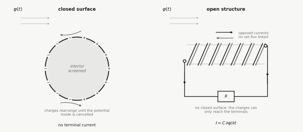
A conductor placed in an external potential does not screen because it is made of copper. It screens because its charges can rearrange into a configuration that cancels the potential inside — and that rearrangement requires somewhere to rearrange to. A closed surface provides it. The induced charges distribute themselves over the enclosure, the interior potential goes flat, and nothing further happens. This is the Faraday cage, and its essential ingredient is the closure, not the metal.
A bifilar coil has two terminals and no closed surface. The charges still move — they must, because their energy reference has shifted — but there is no configuration available to them that cancels the effect. The only route open is toward the terminals. That motion is a current, and a current across a load is a voltage.
Put compactly: the conductor attempts to screen, the attempt cannot complete, and the failure is the signal. The terminal current takes the form
where the capacitance measures how strongly the structure couples to a potential it has no way of expelling. The microscopic account of why conduction electrons respond to a potential at all, in a region where the gauge-invariant fields vanish, is a separate matter and is treated in another article. What matters here is the geometry.
A capacitance that is predicted, not fitted
The coupling capacitance is the sort of quantity that can absorb a discrepancy if it is allowed to. Left as a free parameter it will fit almost anything, and a model that fits by adjustment establishes very little.
It can be estimated instead. The self-capacitance of a single circular loop of wire follows from its radius and the wire gauge — about 0.43 pF per turn for this geometry — and twenty-five turns give a geometric total near 32 pF. The differential winding roughly halves the coupling, since the two conductors of each pair partly shield one another. The prediction is about 15 pF.
The measured geometric capacitance, extracted from the resonance of the receiver circuit with the probe contribution removed, is about 15 pF. The number was not adjusted to make anything agree.
The first test: internal impedance
Varying the load resistance across seven decades, from 0.1 Ω to 1 MΩ, makes the receiver behave as a voltage divider, and the resistance at which the output falls to half its maximum gives the internal impedance of the source. The measurement returns 377 ± 10 Ω.
That number is the impedance of free space, 376.73 Ω, which sits 0.07 per cent from the central value and comfortably inside the interval. Capacitive pickup would not give it: at the operating frequency the reactance of the estimated mutual capacitance is around 4000 Ω, an order of magnitude away. The two hypotheses are not close enough to be confused.
It is worth being clear about what the free-space impedance does and does not indicate. It is the ratio μ₀c, fixed by the propagation speed alone, and it is therefore not a signature of any particular polarisation — a wave travelling at c will present it whatever its mode. Measuring 377 Ω is evidence about a speed, not about a geometry.
The second test: propagation velocity
The speed can also be measured directly, which is the more demanding version of the same question. Twenty-five independent time-delay readings were taken at a separation of 50 cm, triggering on the transmitter channel and timing the arrival at the receiver.
The sample mean is 3.049 × 10⁸ m/s, with a standard deviation of 1.575 × 10⁷ and a 95 per cent confidence interval running from 2.987 to 3.112 × 10⁸ m/s. The accepted value of c lies inside it. The mean sits 1.7 per cent above c, which is well within a measurement whose coefficient of variation is 5.2 per cent.
This is a modest result and should be read as one. It establishes propagation at the speed of light to a precision of a few per cent, which is what a two-channel oscilloscope over half a metre can be expected to deliver. It does not establish anything finer, and the interval is quoted so that it cannot be mistaken for doing so.
The third test: orientation
Orientation is the most direct discriminator available, because different coupling mechanisms make sharply different predictions about it. A response to a changing magnetic field is maximal when the coil axis lies along the flux and vanishes at right angles to it. A response to a vector field aligned with the propagation direction would peak with the coil pointed radially at the source.
Rotating the coil about its centre of mass, holding the centre at 25 cm from the sphere, the received voltage stays within about 5 per cent across every orientation tested. There is no axis of maximum and no null.
One configuration does reduce the signal: laying the coil along the radial direction, near end at 25 cm and far end at 50 cm. But the reduction is expected, and its size follows from geometry with nothing to adjust. In that orientation the potential is not uniform along the coil — it falls as one over distance, from 4.0 V at the near end to 2.0 V at the far end — and the spatial average over the length is
which is 2.77 V, a reduction of 31 per cent. The observed reduction is about 35 per cent. The four points of discrepancy are not accounted for and are recorded as they stand; what matters is that the prediction has no free parameter in it, and that a mechanism responding to a radially directed vector field would have predicted the opposite sign of effect entirely.
A further check replaces the sphere with a hollow aluminium cylinder of comparable size. Rotating the cylinder makes no significant difference to the received signal, which is what one expects if the coupling tracks the total charge on the transmitter rather than the shape of the field around it.
The fourth test: removing the sphere
The three tests so far all interpret a signal. The fourth asks whether the signal is there at all for the reason assumed, and it is the most useful of them because it requires no model to read.
Everything is left connected: the generator running, the feed cable in place along its full length, the receiver where it was, every oscilloscope connection untouched. The only change is the final contact between the cable and the sphere, which is detached. Nothing else in the apparatus moves.
The signal falls to the noise floor.
The strength of the test is in what stays the same. If the reading came from the feed cable radiating, the cable is still there and still driven. If it came from a ground loop, the loop is intact. If it came from pickup along the leads, the leads have not moved. Each of those accounts predicts that detaching the sphere changes nothing, and each is contradicted by a single contact. The test was repeated across several transmitter and receiver configurations with the same outcome.
What the four tests do and do not settle
Taken together they close off the ordinary explanations from four directions. The bifilar winding removes magnetic induction by construction. The impedance measurement separates the response from capacitive pickup by an order of magnitude. The orientation behaviour is inconsistent with both a magnetic and a radially directed vector coupling, and its one departure from isotropy is predicted quantitatively without adjustment. Detaching the sphere eliminates the cable and the wiring as sources.
What survives is a receiver responding to something that arrives at the speed of light, presents the impedance of free space, tracks the charge on the transmitter rather than the geometry of the field, and does not care how the coil is turned.
Several things remain open, and they are worth naming rather than leaving to be discovered. The agreement on the radial reduction is good but not complete, and the residual four points have no account. The behaviour at carrier frequencies approaching the receiver’s own resonance near 35 MHz is predicted to change character, and has not been explored — the measurements reported here all sit in the regime where each response decays fully before the next begins. And the apparatus is a workbench one: a function generator, a sphere, a hand-wound coil and a two-channel oscilloscope. The precision it delivers is the precision such an apparatus delivers, which is a few per cent, and no argument here should be read as resting on more than that.
Sources
S. Filippi, “Local, Causal Field Seeding in Lorenz Gauge via Quaternion Formalism: Longitudinal Scalar Wavefront and Experimental Evidence,” Zenodo, 2026. doi:10.5281/zenodo.21032019
S. Filippi, “Scalar Potential Coupling in Lorenz Gauge: Theoretical Framework and Experimental Evidence,” Zenodo, 2026. doi:10.5281/zenodo.21040664
R. Kubo, “Statistical-Mechanical Theory of Irreversible Processes. I. General Theory and Simple Applications to Magnetic and Conduction Problems,” J. Phys. Soc. Jpn., vol. 12, no. 6, pp. 570–586, 1957.
G. D. Mahan, Many-Particle Physics, 3rd ed. New York: Kluwer Academic/Plenum Publishers, 2000.
Preprints and technical notes are deposited on Zenodo under ORCID 0009-0007-3660-8498.
Open almost any treatment of retarded potentials and you will find, somewhere among the worked examples, a sphere being charged. The potential outside it is written down in one line:
the applied voltage, scaled by distance, delayed by the light travel time. It is the natural first exercise in retardation, and it looks entirely innocent.
There is a question that exercise does not ask, and the answer to it turns out to govern everything else: where is the charge coming from?
Continuity does not negotiate
Start with the conservation of charge, which is not a modelling assumption but a structural feature of electromagnetism:
Integrate it over any volume containing the sphere. The rate of change of the enclosed charge equals minus the current flowing out through the bounding surface. Rearranged: if the enclosed charge is changing, current must be crossing the surface. There is no alternative — not an approximation, not a limit, an identity.
Now impose exact spherical symmetry, which is what makes the potential above take its simple form. A current crossing the surface has a direction. A direction breaks the symmetry.
So the two requirements are incompatible. A perfectly spherically symmetric source whose charge varies in time cannot exist. Not “is difficult to build” — cannot exist, because it would require charge to appear where none was, and nothing in the theory permits that.
This is worth pausing on, because the object in question is not exotic. A time-varying monopole is what one writes down without thinking whenever a charging sphere is treated as spherically symmetric, and it appears in that role in a great deal of otherwise careful work.
Writing it down anyway
Impossible objects can still be written down, and doing so is often instructive: the formalism, asked to describe something that cannot be, tends to say so. What is interesting here is how many different ways it finds to say it.
Take the exterior region seriously as a boundary-value problem. Prescribe the potential above on a spherical boundary, ask for a solution of the wave equation outside it, and impose the Lorenz gauge condition. This is a well-posed mathematical question, whatever its physical status.
The answer is startling. Outside the boundary, while the applied voltage is still changing, the gauge-invariant electric field is exactly zero.
Not small. Zero, identically, at every radius. The magnetic field vanishes by symmetry, and the electric field vanishes because the two terms that make it up cancel term by term:
The gradient of the scalar potential is not zero — it is the ordinary Coulomb-like field one would expect, plus a term proportional to the rate of change of the voltage. But the physical field is that gradient plus the time derivative of the vector potential, and the vector potential required by the Lorenz condition for this source is precisely the one whose time derivative cancels it.
This is not an approximation valid at large distance, or at low frequency, or to leading order. It is an identity, and it has been checked four separate ways: by direct algebraic construction, by the classical equation of motion including the canonical momentum, by the Aharonov–Bohm phase around a closed loop, and by the quantum multipole selection rule, which forbids a monopolar source from emitting a real photon at all because photon emission requires angular momentum a monopole does not have.
A fifth check, using Gauss’s law in the exterior vacuum, is sometimes offered as a fifth proof. It is not one, and it is worth being clear about why. If the field is identically zero then its divergence is zero by construction, so the calculation cannot fail. It verifies that the construction is not internally inconsistent, which is worth knowing, but it does not distinguish a vanishing field from any other divergence-free field in the exterior — including the ordinary Coulomb field.
What the configuration is not
Here is where the impossibility resurfaces, and where the result has to be stated with more care than it first appears to need.
If the exterior field is exactly zero, then the flux of that field through any surface enclosing the boundary is also zero. Gauss’s law in integral form then says the enclosed charge is zero.
But the potential we started from is monopolar, and the coefficient in it is usually read as a charge: the sphere charged to voltage V holds a charge proportional to V. The two statements cannot both be about the same quantity.
The resolution is that the coefficient is a boundary parameter of the retarded solution, not a demonstrated physical charge sitting anywhere. The exterior problem was posed by prescribing a potential on a boundary; it says nothing about the interior, and establishing that the coefficient corresponds to a real surface charge would require solving the interior problem and matching across the boundary. That has not been done, and it is not a formality: for a genuine surface charge the field must be discontinuous across the surface, so a vanishing exterior field would require a non-zero interior field, which a conductor cannot have.
So the configuration with the exactly vanishing exterior field is not a charged conductor. It is an exterior boundary-value problem that carries no net enclosed charge, and the informal phrase “a sphere charged to potential V” should not be read as asserting otherwise.
Three symptoms, one cause
Once this is seen, several separate difficulties turn out to be the same difficulty.
The vector potential constructed above contains the time integral of the applied voltage. If the source settles to a constant voltage, that integral grows without bound, so the constructed vector potential diverges at fixed radius even though the potential itself stays finite. A vector potential growing without limit in a system that has physically reached electrostatic equilibrium is a signal that the solution has stopped being the physical one — it is no longer anchored to a current history, because there is no longer a current.
The flux does not balance, as above
And most directly: applied to a source fed through a single point with no return path included, the Lorenz gauge condition itself is violated substantially. Not marginally — the numbers do not come close. Including an explicit return conductor restores it to within a tenth of a per cent, verified across several dozen field points spanning two decades in distance and the full angular range.
These are not three unrelated problems. They are the impossibility asserting itself at three different places in the formalism: a source whose charge varies without a path for the charge to arrive along is not a solution of Maxwell’s equations, and the machinery says so wherever one happens to look.
There is a moral here about gauge conditions that is easy to miss. The Lorenz condition is usually presented as a convenience, a choice made to decouple the potential equations. It is more than that. Substituted into the field equations it enforces charge conservation, and a source that does not conserve charge cannot satisfy it. What looks like a free choice of bookkeeping is a physical requirement wearing a bookkeeper’s coat.
What the real configuration gives
With the return path included, the comparison can finally be made honestly, and the outcome has two halves that behave quite differently.
The field cancellation degrades, but not by much. The gauge-invariant field is now small rather than exactly zero, tilted away from purely radial by an amount varying systematically with angle relative to the injection point, and the magnetic field is no longer zero. The physical energy flux, identically zero in the idealised problem, becomes non-zero: around 1.7% of the energy stored in the circuit.
Small, genuinely not zero, and it would be wrong to round it down. That figure deserves one qualification. It is a measurement made at a particular place and for a particular transient — five sphere radii out, with the voltage rising over about ten nanoseconds — and it is not a constant of the configuration. Measured further out it grows; measured for a slower transient it shrinks. But the two are not independent: recomputing the geometry by an independent route shows that both collapse onto the single ratio between the size of the system and the distance light travels while the source is rising. Hold that ratio fixed and the deviation holds fixed too, across a factor of sixteen in observation radius.
Which is the more useful statement, because it says what the deviation is measuring. Not a residual inaccuracy, and not a small effect that happens to be there — it is the distance from the quasi-static, written as a ratio of lengths. For a sphere a few centimetres across charged over ten nanoseconds, light crosses the geometry some hundred times during the rise, and a per cent or two is what that buys.
The kinematic identity does not degrade at all. The scalar quantity built from the wavefront of the potential is computable exactly from the behaviour of that potential alone, and the potential of a charged sphere does not depend on how the charge got there. That identity holds unchanged between the idealised and the real configuration.
So two claims that looked equally strong are not equally robust, and the difference is structural rather than a matter of degree. One depends on the currents, and the currents are exactly what a real feed point disturbs. The other depends only on the charge, and a monopole is a monopole however it was assembled.
Why this matters beyond the sphere
The general statement is short. Continuity is not negotiable; what can be chosen is only what carries it.
That reading makes several apparently unrelated situations look the same. A bar of metal polarised by an external field has conduction current that stops at its ends — and the circuit closes through displacement current in the space beyond, which is why the bar radiates while it settles rather than simply arriving at equilibrium. In a high-altitude nuclear detonation, the Compton current streams outward with no return path at all, and the circuit closes because the same electrons ionise the air behind them into a conductor: the source manufactures its own return path while acting, and that process is what limits the pulse.
Three configurations, one rule. In each case the interesting physics is not in the outgoing current, which is obvious, but in how the path closes, which is not.
And it suggests a habit worth keeping. When a calculation involving a time-varying source produces something strange — a quantity growing without bound, a flux that does not balance, a gauge condition that will not hold — the first thing to check is not the algebra. It is whether the charge has somewhere to come from.
Sources
S. Filippi, “Field Exclusion for a Monopolar Source in Lorenz Gauge,” 2026.
S. Filippi, “Dynamic Open-Path Sources and the Lorenz Gauge: Resolving a Charging Sphere with Single-Point Injection,” 2026.
S. Filippi, “The Scalar Longitudinal b-Channel in Lorenz Gauge: Foundations and an Explicit Coulomb-Gauge Verification,” 2026.
C. Galeriu, “The Lorenz gauge condition and charge conservation,” 2022.
J. D. Jackson, Classical Electrodynamics, 3rd ed. New York: Wiley, 1998, Ch. 6.
Y. Aharonov and D. Bohm, “Significance of Electromagnetic Potentials in the Quantum Theory,” Phys. Rev., vol. 115, pp. 485-491, 1959.
Preprints and technical notes are deposited on Zenodo under ORCID 0009-0007-3660-8498.
Late in the evening of 8 July 1962, local time, the streetlights failed along several strings in Oahu. Burglar alarms went off across the islands. A microwave repeater on Kauai stopped working, cutting telephone traffic between Kauai and the other islands. The input stages of ionospheric sounders failed; rectifiers in communication receivers were damaged.
The cause was 1,445 kilometres away, and 400 kilometres up.
At 09:00 UTC on 9 July, a 1.4-megaton device had been detonated above Johnston Island in the Pacific, in a test named Starfish Prime. What reached Hawaii was not blast, not heat, not fallout. It was an electromagnetic pulse — and the instruments deployed to measure it were driven off scale, which is a polite way of saying that the most important measurement of the experiment was lost at exactly the moment it mattered.
This article is about the physics of that pulse, and about how it was worked out afterwards, from a partial record, by people who had guessed wrong the first time.
Two wrong answers
By 1962 there were already models for what a nuclear detonation should do electromagnetically. Neither of them worked.
The first, associated with Hans Bethe, treated the problem as a downward-directed current: charge separation driven radially outward from the burst, with the resulting current radiating. For a burst inside dense air, close to the ground, this is roughly right — the geometry is compact and the radiation is modest. Extrapolated to 400 km, it gave an answer far too small.
The second was the magnetohydrodynamic mechanism: the expanding, highly conductive fireball excludes the geomagnetic field, pushing it aside like a bubble in a fluid, and the field’s subsequent relaxation drives currents in the ionosphere and, by induction, in long conductors on the ground. This is real physics — it does happen, and we will come back to it — but its characteristic timescale is seconds, not nanoseconds. It could not account for a fast, high-amplitude pulse.
Both models failed in the same direction. They underestimated the peak by orders of magnitude. That is worth stating plainly, because the usual account of Starfish Prime presents the EMP as a discovery, when it is more accurately described as the failure of two predictions.
What Longmire saw
The correct mechanism was identified by Conrad Longmire at Los Alamos in 1963, and published in full form much later. The essential move is to stop thinking about the fireball and start thinking about the air, tens of kilometres below it.
A fission or thermonuclear detonation emits a prompt burst of gamma rays. At 400 km altitude there is essentially nothing for them to interact with, so they stream outward in straight lines at c. Moving downward, they eventually reach air dense enough to matter — roughly between 20 and 40 km altitude, where the density is still low by sea-level standards but no longer negligible. This layer is the source region, and it is where all the interesting physics happens.
In the source region, gamma rays Compton-scatter off atomic electrons. The kinematics of Compton scattering at these energies are strongly forward-peaked: the recoil electrons are relativistic and they move, on average, in the same direction the gamma ray was going. So the gamma flux converts itself into an electron flux, propagating radially outward from the burst.
A radial current alone is a poor radiator. What makes this one efficient is the third ingredient, and it was not supplied by the weapon.
The Compton electrons are relativistic charged particles moving through the Earth’s magnetic field, and they are therefore deflected. Whether that deflection matters is a question with a numerical answer, and it is worth working out, because it is what fixes the altitude of the source region.
Two lengths compete. The first is the gyroradius, the scale on which the magnetic field bends the trajectory. For an electron of kinetic energy 1 MeV the momentum is 1.42 MeV/c, and in a field of 30 μT
independent of altitude, since the geomagnetic field barely changes over the first hundred kilometres. The second is the range: how far the electron travels before collisions bring it to rest. This one depends strongly on altitude, because it is a fixed mass per unit area — about 0.44 g/cm2 for a 1 MeV electron — divided by the local air density. At sea level that is 3.6 metres. At 30 km it is 245 metres.
The two cross at 27 km. Below that altitude the electron stops before the field can turn it and the deflection is a negligible correction; above it, the electron completes a substantial arc and the deflection becomes the dominant feature of the trajectory.
That crossing is remarkably insensitive to the electron energy. Quadrupling it, from 0.5 to 2 MeV, moves the crossing only from 30 km to 25.5 km — because gyroradius and range both grow with energy, and the growth largely cancels in the ratio. Which means something worth stating plainly: the altitude of the source region is set by the Earth’s atmosphere and the Earth’s magnetic field. The source has almost no say in it.
Above the crossing, then, the radial current acquires a large transverse component, perpendicular to both the propagation direction and the local field. And a transverse current sheet radiates.
That is the whole mechanism. It is textbook classical electrodynamics — accelerated charge, retarded fields, a current distribution with the right geometry — applied in a configuration nobody had considered because nobody had built one. The radiating structure is a shell of ionized air perhaps thirty kilometres thick and hundreds of kilometres across, illuminated coherently from above by a source at the speed of light. Its effective aperture is enormous, and the Earth’s own magnetic field is one of its components.
Nobody designed it. It assembled itself in a few tens of nanoseconds.
Why it is coherent, and why it saturates
Two features of the geometry deserve attention, because they are what separate this from an ordinary radiation problem.
Coherence. The gamma front travels down at c. The electromagnetic wave produced in the source region also travels at c. An observer on the ground below therefore receives contributions from a large volume of the source region very nearly in phase — the retardation almost exactly cancels the propagation delay of the driving front. The result is constructive addition over a huge radiating volume, and a rise time set not by the size of the structure but by the sharpness of the gamma pulse: nanoseconds. The spectrum is correspondingly broad, which is why the pulse coupled into everything from streetlight strings to receiver front ends.
Saturation. The same Compton electrons that carry the current also ionize the air, and ionized air conducts. The conductivity rises during the pulse and begins to short-circuit the very current that produced it: secondary electrons drift under the induced field in the direction that opposes the primary current.
The equations in this form are due to Karzas and Latter; Longmire’s review presents them with unusual economy. Working in retarded coordinates along the propagation path, and assuming the field varies far more slowly in space than in time, the whole problem collapses onto a single line of sight. What is left is one ordinary differential equation:
where JθC and Eθ are the transverse components of the Compton current density and of the field, σ the rising conductivity of the ionized air, and Z0 = 377 Ω the impedance of free space. There is a second, identical equation for the φ component; the two are linked by Bθ = −Eφ and Bφ = Eθ, which is why the free-space impedance appears here at all — it is not a fitted coefficient but μ0c, arriving on its own.
The derivative is not dE/dz but (1/r)·∂(rE)/∂r, and the difference matters: the 1/r is the wavefront spreading as it goes. The antenna is growing while it radiates.
One equation, and it contains both the source and the mechanism that extinguishes it.
The consequence is immediate. The field stops growing when the bracket vanishes,
so the pulse is capped not by how much current is produced but by how fast the medium becomes conducting. Setting the two terms equal over a path length L gives a threshold conductivity of order σ ≈ 2/(Z0L). Read that as a statement about impedance rather than about conductivity, and it says something clean: the source region shorts itself out when its sheet conductance reaches the admittance of free space. It is impedance matching, running in reverse — the same 377 Ω that governs how efficiently an antenna couples to empty space, here setting the ceiling on how large the pulse can become.
This is why the peak does not scale indefinitely, and why above a certain point additional gamma output buys nothing. The pulse is bounded by the electrodynamics of the medium, not by the source.
Three pulses, not one
Modern practice distinguishes three components, labelled E1, E2 and E3. The taxonomy is a later formalization — it is not the language of 1962 — but it is a genuine physical distinction, because the three arise from different mechanisms on timescales separated by many orders of magnitude.
E1 is the Compton–geomagnetic mechanism just described: nanosecond rise, tens of nanoseconds duration, high field amplitude, broad spectrum. It couples to anything with a dimension comparable to its wavelengths — cables, antennas, circuit traces.
E2 is the intermediate-time component, driven by scattered gamma rays and by neutron-induced reactions, extending into the microsecond–millisecond range. Its characteristics resemble a lightning strike, which is why it is the least troublesome: existing protection was designed for exactly this.
E3 is the slow one, and it is the MHD mechanism from the second failed model — not wrong, merely a different phenomenon. Timescale: seconds to minutes. It is functionally an artificial geomagnetic storm, and like a natural one it induces quasi-DC currents in very long conductors — power lines, pipelines, telegraph cables.
The clearest evidence for E3 does not come from Starfish Prime. On 22 October 1962 the Soviet Union conducted a high-altitude test over Kazakhstan, part of the series later known in the West as Project K. The yield was far smaller than Starfish — a few hundred kilotons — but the burst was over a large populated landmass at a higher geomagnetic latitude, and the ground below was crossed by long buried power lines. The induced surge started a fire in a power plant at Karaganda.
That result was not available outside the Soviet Union for three decades. It became known to Western researchers only after 1991, when Russian scientists were able to publish on the subject. It is a useful reminder of what the empirical base for this field actually consists of: a small number of experiments, unevenly instrumented, unevenly reported, conducted over about five years.
The other half: belts
The pulse was not the only thing Starfish Prime left behind, and the second effect had been predicted correctly — by someone who was not, formally, a physicist.
Nicholas Christofilos, at what is now Lawrence Livermore, had proposed in 1957 that beta electrons from the decay of fission fragments, released above the atmosphere, would be captured by the geomagnetic field. The argument rests on the adiabatic invariants of charged-particle motion: an electron on a field line spirals, mirrors near the poles where the field is strong, and drifts in longitude, so that within a few minutes an initially localized injection smears into a shell encircling the planet. Christofilos was reasoning by analogy with the radiation belts James Van Allen had just discovered with Explorer I.
The idea was tested with unusual speed. Explorer IV was instrumented by Van Allen’s group and launched on 26 July 1958. Three small devices were detonated at high altitude over the South Atlantic on 27 August, 30 August and 6 September 1958, launched by rocket from the USS Norton Sound: Operation Argus. The prediction held. An artificial electron shell formed, was detected from orbit, and decayed over several weeks.
Starfish Prime, four years later, was three orders of magnitude larger, and the resulting belt did not decay over weeks.
Telstar
The quantitative record here is better than for the pulse, because the instruments did not saturate — they simply degraded, and the degradation was logged.
TRAAC and Transit 4B had been launched together in November 1961 into the same orbit, and both carried circuits monitoring their own solar cell output. Between launch and 9 July 1962 they had lost 17% and 18% of initial output respectively, from natural radiation. After Starfish Prime, Transit 4B lost a further 22% in twenty days, and TRAAC 22% in twenty-eight. Transit 4B stopped transmitting on 2 August 1962; TRAAC on 14 August.
This is a clean before-and-after in a single instrument, and it is the most convincing single dataset on the artificial belt.
Ariel 1, the first British satellite, lost solar array performance and never fully recovered. Injun 1 and the Soviet Kosmos 5 were degraded. Telstar 1 — the first active communications satellite, launched on 10 July 1962, one day after the test, into an orbit that repeatedly crossed the new belt — suffered transistor damage in its command decoder and failed permanently in February 1963, seven months into a mission that had been expected to last considerably longer.
Roughly one third of the two dozen or so satellites then in low orbit were damaged or destroyed. The belt itself persisted for years; estimates of a decade or more appear in the literature.
Whether Telstar’s failure should be attributed to Starfish Prime rather than to the natural belt is a question that has been revisited more than once, and the attribution rests on the timing and on the dose reconstruction rather than on a direct measurement. It is generally accepted, but it is an inference.
What the record actually supports
The Limited Test Ban Treaty of August 1963 closed the laboratory. Everything we know empirically about high-altitude nuclear electromagnetic effects comes from before that date, from a handful of shots, several of which were — in the words of the project officer’s own report on Starfish — poorly instrumented and hastily executed, with models too uncertain to permit extrapolation to other altitudes and yields with any confidence.
That assessment was written to justify Starfish Prime. It applies almost as well afterwards.
The peak E1 field at Hawaii is a reconstruction. The primary records saturated; the values quoted in the literature are inferred from the few unsaturated channels, from damage thresholds, and from later modelling. The mechanism is not in doubt — Longmire’s account is solid, and it is ordinary electrodynamics — but the numbers attached to it are model-dependent in a way that is not always made explicit in secondary sources.
The crossover altitude quoted above is my own calculation, not a figure taken from the literature: electron ranges from the ESTAR tabulation, air density from the US Standard Atmosphere of 1976, and a representative geomagnetic field of 30 μT. The 20–40 km source region is standard; the 27 km crossing is simply where those three inputs put it.
Modelling has continued. As recently as 2022, a three-dimensional simulation at Lawrence Livermore reproduced the 1962 magnetometer records from first principles for the first time, and in doing so split the E3 component into two distinct behaviours depending on whether the signal passes through or around the X-ray ionization patch. Sixty years after the experiment, the interpretation of the data is still being refined.
There is something instructive in that. The physics here involves no new principle: Maxwell’s equations, Compton scattering, the Lorentz force, adiabatic invariants. Every ingredient was known by 1930. What was missing was the recognition that a particular geometry — a coherently illuminated conducting shell in a magnetized medium — would behave as an antenna of extraordinary efficiency. The configuration had to be built by accident before anyone thought to analyse it, and once it had been built twice, it was made illegal.
We are left studying, for sixty years and counting, a handful of measurements from an experiment that cannot be repeated.
Sources
C. L. Longmire, “On the electromagnetic pulse produced by nuclear explosions,” IEEE Trans. Electromagn. Compat., vol. EMC-20, no. 1, pp. 3–13, Feb. 1978. Joint Special Issue on the Nuclear Electromagnetic Pulse, published concurrently with IEEE Trans. Antennas Propag., vol. AP-26, no. 1, Jan. 1978.
W. J. Karzas and R. Latter, “Detection of the electromagnetic radiation from nuclear explosions in space,” Phys. Rev., vol. 137, no. 5B, pp. B1369–B1378, 1965.
H. Hoerlin, United States High-Altitude Test Experiences: A Review Emphasizing the Impact on the Environment, LA-6405, Los Alamos Scientific Laboratory, 1976.
S. Glasstone and P. J. Dolan, The Effects of Nuclear Weapons, 3rd ed. Washington, DC: U.S. Department of Defense and Department of Energy, 1977, Ch. 11.
N. C. Christofilos, “The Argus experiment,” J. Geophys. Res., vol. 64, no. 8, pp. 869–875, 1959.
J. A. Van Allen, C. E. McIlwain, and G. H. Ludwig, “Satellite observations of electrons artificially injected into the geomagnetic field,” J. Geophys. Res., vol. 64, no. 11, pp. 1683–1696, 1959.
P. J. Edwards and S. A. Reid, J. Geophys. Res., vol. 69, no. 17, pp. 3607–3612, 1964.
T. I. Gombosi, D. N. Baker, A. Balogh, P. J. Erickson, J. D. Huba, and L. J. Lanzerotti, “Anthropogenic space weather,” Space Sci. Rev., vol. 212, pp. 985–1039, 2017.
M. J. Berger et al., ESTAR: Stopping Powers and Range Tables for Electrons, NIST Standard Reference Database 124.
R. E. Fischell, solar cell degradation measurements on TRAAC and Transit 4B, Applied Physics Laboratory, 1962.
U.S. Government Project Officer’s Interim Report on Starfish Prime, Joint Task Force 8, 1962.