Author: stfi66

  • One Operator, Four Domains

    The previous article ended on an algebraic observation: quaternion multiplication produces the dot and cross products together, from a single operation, because neither was put in by hand. What follows is what happens when that multiplication is applied to a derivative.

    The result is one differential operator that, applied without modification to four unrelated physical quantities, returns four unrelated sets of known equations. None of this is new physics and none of it is claimed to be. What is worth setting out is the mechanism, and — equally — where it stops.

    First, a complication

    Real quaternions are not quite enough. The norm established earlier is a sum of four squares, and therefore positive whatever the components are. Relativity needs something else: the spacetime interval carries the time part with the opposite sign from the three space parts, and no sum of squares does that.

    The standard remedy, already used by Minkowski, is to let the coefficients be complex rather than real. The result is a biquaternion:

    Q~=w+xi+yj+zk,w,x,y,z∈ℂ\tilde{Q} = w + x\,i + y\,j + z\,k, \qquad w,x,y,z \in \mathbb{C}

    The complexifying unit is written in bold, i, to keep it distinct from the Hamiltonian unit i. It squares to −1 like the others, but unlike them it commutes with everything.

    Two things follow that are worth stating once and not revisiting. Biquaternions are no longer a division algebra — the guarantee that every non-zero element has an inverse is lost, and there exist non-zero elements whose product is zero. And there are now two distinct conjugations, because there are two kinds of imaginary unit to flip:

    Q~∗=w−xi−yj−zk,Q~∗=w∗+x∗i+y∗j+z∗k\tilde{Q}^{*} = w – x\,i – y\,j – z\,k, \qquad \tilde{Q}_{*} = w^{*} + x^{*}i + y^{*}j + z^{*}k

    The superscript asterisk flips i, j, k and leaves the coefficients alone; the subscript flips i and leaves i, j, k alone. With real coefficients the two coincide, which is why the previous article needed only one of them.

    The point of the complication shows up immediately. Write the spacetime position as a biquaternion with an imaginary time component, and form the product with its conjugate:

    X~=𝐢ct+𝐗,X~X~∗=c2t2−X12−X22−X32\tilde{X} = \mathbf{i}\,ct + \mathbf{X}, \qquad \tilde{X}\tilde{X}_{*} = c^2t^2 – X_1^2 – X_2^2 – X_3^2

    which is the Minkowski interval, invariant under Lorentz transformations. The mechanism is the one from before — the cross-product term dies because a vector’s cross product with itself vanishes — but the sign structure is now right.

    The operator

    Everything that follows uses one object, unchanged:

    ∇~=𝐢c∂∂t+∇\tilde{\nabla} = \frac{\mathbf{i}}{c}\frac{\partial}{\partial t} + \nabla

    A time derivative in the scalar slot, the gradient in the vector slot. Nothing has been assumed about what it will act on.

    Now apply the self-conjugate product to the operator itself. The cross-product term vanishes for the same reason it always does — here because mixed partial derivatives commute, so the formal curl of the gradient is identically zero — and what is left is purely scalar:

    ∇~∇~∗=1c2∂2∂t2−∇2\tilde{\nabla}\tilde{\nabla}_{*} = \frac{1}{c^2}\frac{\partial^2}{\partial t^2} – \nabla^2

    That is the wave operator, up to a sign. Fixing the sign to match the usual convention:

    ∇~2≡∇~∇~∗=1c2∂2∂t2−∇2=□\tilde{\nabla}^{2} \equiv \tilde{\nabla}\tilde{\nabla}_{*} = \frac{1}{c^2}\frac{\partial^2}{\partial t^2} – \nabla^2 = \Box

    The d’Alembertian, built out of nothing but the multiplication rule. This single fact is the reason the operator works in the domains below, and — as the last section makes explicit — the reason it fails outside them.

    Energy and momentum

    Build a biquaternion from energy and momentum, with the same structure as the spacetime one:

    P~=𝐢cE+𝐩,E=γmc2,𝐩=γm𝐯\tilde{P} = \frac{\mathbf{i}}{c}E + \mathbf{p}, \qquad E = \gamma m c^2, \quad \mathbf{p} = \gamma m \mathbf{v}

    and the identical computation returns the relativistic invariant m²c², equivalent to the familiar relation between energy, momentum and rest mass.

    More interesting is to apply the operator once and set the result to zero — the statement that the system is closed. Reading E and p as local densities in a continuum rather than as properties of a single particle, the product expands into three algebraically independent parts, and each must vanish separately.

    The real scalar part gives local energy-momentum continuity:

    1c2∂E∂t+∇⋅𝐩=0\frac{1}{c^2}\frac{\partial E}{\partial t} + \nabla\cdot\mathbf{p} = 0

    The imaginary vector part gives Newton’s second law in density form, with the gradient of the energy density playing the part of a force density:

    ∂𝐩∂t=−∇E\frac{\partial \mathbf{p}}{\partial t} = -\nabla E

    And the real vector part gives

    ∇×𝐩=0\nabla \times \mathbf{p} = 0

    This third one deserves attention, because it is not automatically satisfied. It is a genuine restriction: the construction reconstructs energy-momentum conservation only for irrotational momentum fields. Rotational configurations are outside what this particular case can describe, and saying so is part of stating the result honestly.

    One further consequence is worth extracting. Integrating the continuity relation over a control volume, and noting that the integral of the momentum divergence has the dimensions of mass, gives mass–energy equivalence — not posited separately, but as a consequence of local conservation.

    The same object, read as a fluid

    Now change nothing about the operator and almost nothing about the quaternion. Take the non-relativistic limit, relabel the mass variable as a density, and read the object as describing a small parcel of ordinary fluid.

    A fluid parcel under gravity is not a closed system, so the right-hand side need no longer be zero. Writing the source as a biquaternion built from the gravitational force density and a vorticity term, the same three-part decomposition returns three familiar results.

    The real scalar part gives mass continuity. The imaginary vector part, identifying the scalar with the fluid pressure, gives Euler’s equation for a perfect fluid:

    ∂𝐯∂t=𝐠−1ρ∇P\frac{\partial \mathbf{v}}{\partial t} = \mathbf{g} – \frac{1}{\rho}\nabla P

    And the real vector part — the slot that the closed case was forced to set to zero — now carries the vorticity of the mass flow. The irrotationality restriction flagged above was never a limitation of the algebra. It was a consequence of assuming no source; introducing one releases it.

    Two caveats belong here rather than in a footnote. The identification of the scalar with pressure is an external physical input, not something the algebra supplies. And because the operator is linear, the construction produces only the local time derivative, never the full material derivative of the general Euler equation — the convective term is genuinely nonlinear in the velocity, and nothing a linear operator applied once can generate accounts for it.

    Linearising around a fluid at rest and introducing a velocity potential, one further application of the same operator — built with the speed of sound in place of the speed of light — returns the acoustic wave equation directly, with no machinery beyond what was already assembled.

    Quantum mechanics, partly

    The relativistic invariant from the energy-momentum section is also where relativistic quantum mechanics begins. Quantising it in the standard way and applying the result to a wavefunction gives the Klein–Gordon equation, which by the d’Alembertian identity above is exactly

    ∇~2ψ=−(mcℏ)2ψ\tilde{\nabla}^{2}\psi = -\left(\frac{mc}{\hbar}\right)^{2}\psi

    the same operator, applied now to a wavefunction rather than to a spacetime or momentum quaternion.

    There is a second and more delicate connection, this one concerning the Hamiltonian units themselves. Dirac’s construction requires four objects that anticommute with one another and square to plus one. The Hamiltonian units anticommute correctly but square to minus one — the wrong sign. Multiplying each by the complexifying unit fixes it exactly:

    αk≡𝐢ek,αk2=𝐢2ek2=(−1)(−1)=+1\alpha_k \equiv \mathbf{i}\,e_k, \qquad \alpha_k^{2} = \mathbf{i}^{2}e_k^{2} = (-1)(-1) = +1

    and three of Dirac’s four objects are reproduced.

    The fourth is not, and cannot be. The biquaternion algebra is eight-real-dimensional, and once the three units above are identified, that space is already fully spanned; there is no room left for an independent fourth generator with the required properties. Completing the Dirac equation needs the larger sixteen-dimensional Clifford algebra. What the quaternions reproduce is a genuine part of that structure, and not the whole of it.

    Where it stops

    Four domains, one operator, no modifications. It would be easy to present this as evidence of some deep universality. It is not, and the reason is visible in the construction itself.

    The square of the operator is the d’Alembertian, by construction. That makes it intrinsically hyperbolic: second order in time, symmetric under time reversal, propagating disturbances at a finite speed. Every domain above shares exactly that skeleton. Four-momentum conservation, the Euler equations, Klein–Gordon — all wave-like, all second order in time.

    Heat conduction is not. The diffusion equation is first order in time and parabolic; it distinguishes past from future, and it does not follow from this operator applied to any natural quaternion built from temperature and heat flux. No relabelling of variables changes that, because the obstruction is structural rather than notational.

    So the honest statement of the result is narrower than the list of four domains suggests, and the narrowness is the substance of it. The operator does not reconstruct physics in general. It reconstructs the physics that is already wave-like — which is a real and non-obvious fact about a large part of theoretical physics, and nothing more than that.

    One domain has been left out of this article deliberately: electromagnetism, where the same operator does something the others do not.


    Sources

    • P. A. M. Dirac, “The Quantum Theory of the Electron,” Proc. R. Soc. Lond. A, vol. 117, pp. 610–624, 1928.
    • A. W. Conway, “On the applications of quaternions to some recent developments of electrical theory,” Proc. R. Ir. Acad., vol. 29, pp. 1–9, 1911.
    • L. Silberstein, “Quaternionic form of relativity,” Phil. Mag., vol. 23, pp. 790–809, 1912.
    • A. Gsponer and J.-P. Hurni, “The Physical Heritage of Sir W. R. Hamilton,” arXiv:math-ph/0201058.
    • R. J. Nagem, C. Rebbi, G. Sandri, and S. Shei, “Gauge transformations and local conservation equations for linear acoustics and for Maxwell’s equations,” Nuovo Cimento B, vol. 113, pp. 1509–1517, 1998.
  • The Algebra Hamilton Was Looking For

    Complex numbers work because they are closed. Multiply two of them and you get a third; the operation never takes you outside the system. That closure is what makes them useful for rotations in a plane, and it is why they turn up everywhere in two-dimensional problems.

    The obvious next question is whether the same trick works in three dimensions. William Rowan Hamilton spent something like thirteen years on it. The answer, which cost him those years, is that it does not — and that the case which does work is four-dimensional.

    What follows is what he found, and why the structure is stranger than it first appears.

    The multiplication rule

    A quaternion has four real components and three distinct imaginary units:

    Q~=a+bi+cj+dk,a,b,c,d∈ℝ\tilde{Q} = a + b\,i + c\,j + d\,k, \qquad a,b,c,d \in \mathbb{R}

    The units obey a single compact rule, the one Hamilton carved into Broom Bridge in Dublin on 16 October 1843:

    i2=j2=k2=ijk=−1i^2 = j^2 = k^2 = ijk = -1

    Everything else follows from it. Each unit squares to −1, as the ordinary imaginary unit does. But taken in pairs they behave in a way that has no counterpart in the complex numbers:

    ij=k,jk=i,ki=jji=−k,kj=−i,ik=−j\begin{aligned} ij &= k, & jk &= i, & ki &= j \\ ji &= -k, & kj &= -i, & ik &= -j \end{aligned}

    Read the second line carefully. The order matters. Multiplying i by j does not give the same answer as multiplying j by i — it gives the opposite sign.

    This is the property that makes quaternions worth the trouble, and also the reason they are unfamiliar. Ordinary numbers commute. Complex numbers commute. Quaternions do not, and any intuition built on the assumption that xy equals yx fails here immediately.

    Splitting the object in two

    It is convenient to separate a quaternion into two parts of different character: a single real number, and the three components carrying the imaginary units.

    Q~=q0+𝐐,q0=a,𝐐=bi+cj+dk\tilde{Q} = q_0 + \mathbf{Q}, \qquad q_0 = a, \quad \mathbf{Q} = b\,i + c\,j + d\,k

    Written this way, Q can be identified with an ordinary vector in three-dimensional space, with components b, c, d. So a quaternion is a scalar and a vector, carried together in one object rather than treated as two separate things.

    Addition is unremarkable: the scalars add, the vectors add, and multiplication by an ordinary real number scales both. It is multiplication where something happens.

    The product, worked out

    Take two quaternions with no scalar part at all — two pure vectors, P and Q — and multiply them using nothing but the rule above.

    The expansion has nine terms. Three of them pair a unit with itself, and each contributes a factor of −1: these produce −P₁Q₁, −P₂Q₂, −P₃Q₃. Together they are minus the dot product, and being products of real numbers they carry no imaginary unit — they are a pure scalar.

    The remaining six pair different units, and this is where the anticommutation earns its keep. The pair ij gives k, the pair ji gives −k; collecting them leaves a difference of products rather than a sum. That difference is exactly the cross product.

    The result:

    𝐏𝐐=−𝐏⋅𝐐+𝐏×𝐐\mathbf{P}\mathbf{Q} = -\,\mathbf{P}\cdot\mathbf{Q} \;+\; \mathbf{P}\times\mathbf{Q}

    One multiplication. Two familiar operations, both produced at once, from an algebra in which neither was put in by hand. The dot product falls out of the squares of the units; the cross product falls out of their refusal to commute.

    For quaternions with scalar parts as well, the general product is

    P~Q~=p0q0−𝐏⋅𝐐+p0𝐐+q0𝐏+𝐏×𝐐\tilde{P}\tilde{Q} = p_0 q_0 – \mathbf{P}\cdot\mathbf{Q} + p_0\mathbf{Q} + q_0\mathbf{P} + \mathbf{P}\times\mathbf{Q}

    and the non-commutativity is now visible in one place: every term is symmetric under exchange of the two factors except the cross product, which changes sign. Two quaternions commute only when their vector parts are parallel.

    Why four dimensions and not three

    What Hamilton wanted was not merely a system where multiplication is defined, but one where it can be undone: an algebra in which every non-zero element has an inverse, so that division always works. That is a strong requirement, and it is the reason three dimensions fail.

    Define the conjugate by flipping the sign of the vector part alone:

    Q~∗=q0−𝐐\tilde{Q}^{*} = q_0 – \mathbf{Q}

    and multiply a quaternion by its own conjugate. In the general product above, the cross-product term becomes Q × (−Q), which vanishes identically — any vector’s cross product with itself is zero. The scalar-vector terms cancel against each other. What survives is purely scalar:

    Q~Q~∗=Q~∗Q~=q02+𝐐⋅𝐐=a2+b2+c2+d2≥0\tilde{Q}\tilde{Q}^{*} = \tilde{Q}^{*}\tilde{Q} = q_0^{2} + \mathbf{Q}\cdot\mathbf{Q} = a^2 + b^2 + c^2 + d^2 \;\geq\; 0

    a sum of four squares, and therefore zero only when every component is zero. This gives the norm, and with it the inverse:

    Q~|=Q~Q~∗,Q~−1=Q~∗|Q~|2\tilde{Q}| = \sqrt{\tilde{Q}\tilde{Q}^{*}}, \qquad \tilde{Q}^{-1} = \frac{\tilde{Q}^{*}}{|\tilde{Q}|^{2}}

    Every non-zero quaternion can be divided by. Along with the real numbers and the complex numbers, this makes quaternions one of a very short list — and Frobenius later proved the list is complete for associative algebras over the reals. There is no five-dimensional version, no seven. The four-dimensional case is not one option among many; it is the last one available.

    The mechanism behind that calculation is worth keeping in view, because it recurs: anything times its own conjugate collapses to a pure scalar, because a vector’s cross product with itself always vanishes. It is a small fact, and a good deal rests on it.

    A picture, and what it hides

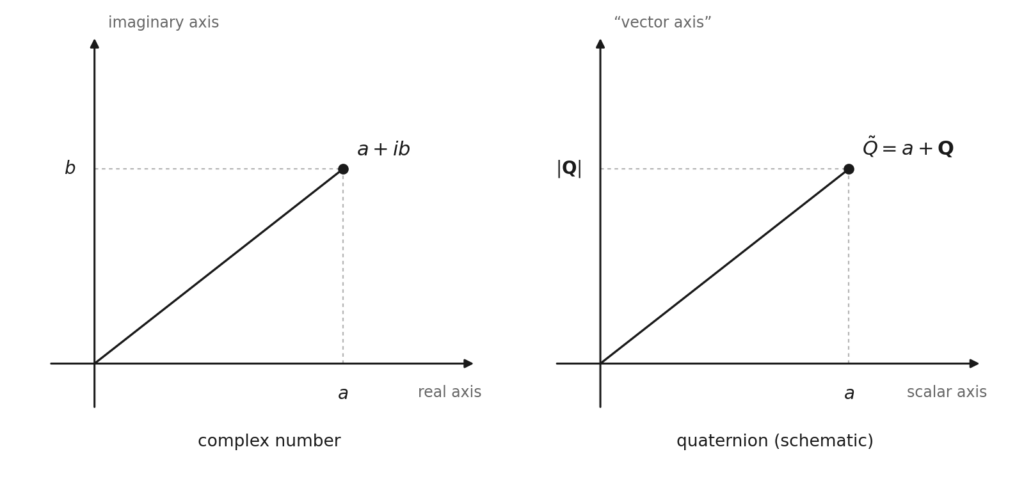
    The figure is a mnemonic, not a diagram of the structure. A complex number splits into a real and an imaginary coordinate; a quaternion splits into a scalar and a vector part, and plotting the magnitude of that vector part on a single axis reproduces the right relationship for the norm, since

    |Q~|2=a2+|𝐐|2|\tilde{Q}|^{2} = a^{2} + |\mathbf{Q}|^{2}

    depends on Q only through its magnitude, exactly as the modulus of a complex number depends only on b.

    Two things are hidden rather than simplified, and both matter.

    The direction of Q is gone. Compressing three components onto one axis keeps the magnitude and discards everything else, and no amount of redrawing fixes this: adding a third axis would recover two of the three components and arbitrarily privilege them over the third. What is needed is not another axis but a change of kind — the vector part promoted to a genuine three-dimensional subspace, with the scalar carried as a fourth coordinate alongside it. That is a four-dimensional object, and it cannot be drawn.

    And the non-commutativity is invisible. Nothing a two-dimensional picture can suggest reproduces the actual product, because the picture has no way to express that the order of multiplication changes the answer. The figure is authoritative on the norm, and on nothing else.

    What the algebra is good for

    The immediate application, and the one still in daily use, is rotation. Unit quaternions represent rotations in three-dimensional space without the degenerate configurations that afflict angle-based descriptions, and they compose by multiplication. Computer graphics, robotics and spacecraft attitude control all run on this.

    But the property that matters for physics is the one that came out of the product above. In the vector calculus that replaced quaternions in the 1880s, the dot product and the cross product are two separate operations, defined independently, with no structural relation to each other. In quaternion algebra they are two parts of a single multiplication — and any product of two quaternions carrying vector parts necessarily generates both.

    That is a statement about algebra, not about physics, and nothing here claims otherwise. But it is worth noticing that a formalism which cannot produce one without the other will behave differently, when applied to a physical problem, from one in which the two are separate by construction.


    Sources

    • W. R. Hamilton, “On quaternions,” Proc. R. Irish Acad., vol. 3, pp. 1–16, 1847.
    • G. Frobenius, “Über lineare Substitutionen und bilineare Formen,” J. Reine Angew. Math., vol. 84, pp. 1–63, 1878.
    • A. Gsponer and J.-P. Hurni, “The Physical Heritage of Sir W. R. Hamilton,” arXiv:math-ph/0201058.
  • What the Electrons Respond To

    A conducting sphere is charged, and in the region outside it the electromagnetic field is exactly zero — no electric field, no magnetic field, no Poynting flux — for as long as the charging lasts. A receiver placed in that region nevertheless produces a measurable voltage, arriving at the speed of light.

    The first half of that has been established elsewhere, along with the considerable qualifications it requires. This article is about the second half: what the receiver is responding to, given that there is nothing there to push its electrons around.

    The route that leads nowhere

    The obvious place to start is the classical equation of motion. A conductor responds to fields; write the force on a conduction electron and see what it gives.

    It gives zero. The Lorentz force is the charge times the electric field plus the velocity cross the magnetic field, and both fields vanish. The equation is satisfied identically, for an electron of any velocity, at every point and every instant.

    That is not a difficulty to be worked around. It is correct, and it is the whole content of the classical level: no force, no classical dynamics. An identity of the form nothing equals nothing determines nothing, and no amount of care in solving it will produce a mechanism.

    So the classical equation of motion is the wrong instrument. It is not that it gives the wrong answer — it gives no answer, and says so honestly.

    Where the coupling actually lives

    The right instrument is the Hamiltonian, and the reason is worth stating in general terms before looking at this particular case.

    The relation between a force balance and a Hamiltonian is the relation between statics and analytical mechanics. Knowing that the normal force on a block equals its weight tells you nothing about how a constrained system moves; the dynamics come from the Lagrangian or the Hamiltonian, and they contain terms that no force diagram displays. The same asymmetry applies here, and it is the standard structure of mechanics rather than anything peculiar to this problem.

    Written out for a conduction electron in the Lorenz gauge, the minimal-coupling Hamiltonian is:

    H=p^22m−qm𝐀⋅p^+iℏq2mb+q2A22m+qφH = \frac{\hat{p}^2}{2m} – \frac{q}{m}\mathbf{A}\cdot\hat{p} + \frac{i\hbar q}{2m}b + \frac{q^2 A^2}{2m} + q\varphi

    Four terms beyond the free kinetic energy. The last of them is the one that matters, and the crucial point about it is structural: the term involving the scalar potential is not part of the kinetic sector. It does not descend from the momentum operator, it is not what generates the Lorentz force, and it does not vanish when the fields vanish. It sits there as long as the potential is non-zero, whatever the fields are doing.

    What it does, in a conductor, is shift the electrochemical potential:

    μ=EF+qφ(t)\mu = E_F + q\varphi(t)

    uniformly across the receiver. Every conduction electron finds its energy reference displaced, in step, by an amount that tracks the potential in time.

    What happened to the other three terms

    This is where the argument could easily have gone wrong, and where checking it changes the answer.

    Two of the remaining terms — the paramagnetic and the diamagnetic — are exactly the ones a bulk conductor usually picks up, and they involve the vector potential, which is emphatically not zero here. A first estimate, taking the paramagnetic term alone against a single-electron energy scale, suggested they might contribute a per cent or a few per cent of the response.

    That estimate does not survive the correct treatment, and the reason it fails is instructive. In any bulk conduction response, gauge invariance of the conductivity — expressed through the f-sum rule, standard in linear response theory — forces the paramagnetic and diamagnetic terms to combine. They cannot appear separately in an observable. What they combine into is a response that depends only on the physical field:

    jbulk(ω)=σ(ω)E(ω)≡0because 𝐄tot≡0j_{bulk}(\omega) = \sigma(\omega) E(\omega) \equiv 0 \qquad \text{because } \mathbf{E}_{tot} \equiv 0

    and the physical field is identically zero throughout the dynamic regime. So the bulk conduction current is not one to four per cent. It is exactly zero — the same null result as at the classical level, now extended from the Lorentz force to the entire bulk-conduction channel, paramagnetic and diamagnetic terms included.

    The estimate was superseded rather than confirmed, and the correction went in the direction of strengthening the null result rather than weakening it. Recording that matters more than the number: an approximate answer of one to four per cent and an exact answer of zero are different kinds of statement, and the second is the one that stands.

    The fourth term, the non-Hermitian one, is bounded separately and comes out around one part in a million. It is not the mechanism either.

    What the electrons respond to

    That leaves the potential term, and the question of how it produces a current. Here the linear-response machinery has to be applied with some care, because the natural way to set it up gives nothing.

    Standard practice couples the perturbation to the electric field and computes the current response. Do that here, in the long-wavelength limit appropriate to a receiver small compared to the distances involved, and the answer vanishes — consistently with the field being zero, and uselessly. That route is not wrong, it is empty. It cannot be used.

    The physically correct route couples the perturbation to the charge density instead, which is to say to the potential itself rather than to its gradient. The response function obtained that way remains finite in the same limit. And the physical reading of that statement is the point of the whole exercise:

    The electrons are not responding to a spatial gradient of the potential across the receiver. To leading order there is none — the potential is essentially uniform over the device. They are responding to the change in time of their own local electrochemical potential.

    That is an ordinary mechanism. It is classical linear response of the Kubo–Drude kind, the same machinery used for conductivity in metals, with a relaxation time in the tens of femtoseconds — nine orders of magnitude faster than the transients involved. Nothing exotic is being invoked. What is unusual is only the perturbation it is being applied to.

    The agent and the condition

    One distinction deserves to be made explicit, because the two halves of it are easy to conflate and they are not the same statement.

    The agent is the potential itself, not its rate of change. The coupling term in the Hamiltonian contains the potential, and it is present whenever the potential is non-zero, whether or not it is changing. A constant potential still shifts the electrochemical potential and still displaces the equilibrium charge distribution of the conductor accordingly.

    What a constant potential does not do is sustain a current. The displaced distribution, once reached, is stationary — the conductor equilibrates to its new reference and then nothing further happens.

    The rate of change enters only through continuity:

    ∂ρ∂t+∇⋅𝐉=0\frac{\partial \rho}{\partial t} + \nabla \cdot \mathbf{J} = 0

    If the charge density at a point is changing, a current must flow. So a non-zero rate of change is what turns a one-off equilibration into a continuing, measurable current — the condition under which a receiver can register the effect, rather than a second mechanism competing with the first.

    Two levels of the same physics: the coupling in the Hamiltonian, and the observability enforced by continuity. Not two rival explanations.

    What the bookkeeping quantities are, and are not

    A programme of this kind accumulates derived quantities — a scalar built from the divergence of the vector potential, an energy density formed from it, a flux, several integrated energies. It is worth being blunt about their status, because the temptation to promote them is real and the discipline against it is what keeps the account honest.

    None of them is independent physical energy, flux, or radiated power.

    The scalar quantity itself is gauge-dependent by construction: it vanishes identically in Coulomb gauge, which is enough to settle the question on its own. The energy density and flux built from it are local diagnostics, and where they are non-trivial the ordinary electromagnetic stress-energy tensor is identically zero — so there is nothing for them to be carrying. Several of the integrated quantities numerically anticipate a physical energy, which is a useful property and not the same as being one. Others turn out to be local re-expressions of circuit power that has already been counted once at the terminals; counting it twice would be an error, not a discovery.

    Exactly one quantity in the family is physical field energy, and it is the settled electrostatic energy after the transient is over.

    What all the others share is a single common status, and it is better stated once than corrected six times: they are gauge-dependent diagnostics of where and when the physical process is active — that process being the potential coupling in the Hamiltonian, and nothing else. A diagnostic that tells you accurately when something is happening is worth having. It is not the thing that is happening.

    Not an Aharonov–Bohm effect

    The comparison is unavoidable and should be made carefully, because the resemblance is real and the identification would be wrong.

    Aharonov and Bohm established that a potential can have observable consequences in a region where the gauge-invariant field vanishes. That principle is what is at work here too, and the debt should be acknowledged.

    But the scalar version of their effect requires the electric field to vanish at the location of the charge, which is achieved with a Faraday-shielded enclosure, and the observable is a quantum phase shift measured by interference. Here the geometry is open and unshielded, a particular field quantity at the receiver is not zero, and the mechanism is classical linear response producing a terminal voltage — no interference, no phase measurement, no shielding.

    Same principle, different mechanism. Not a macroscopic reproduction, and describing it as one would be an overstatement that the details do not support.

    What remains open

    One structural question in this account is not settled. The construction of the vector potential used throughout is argued to be the unique causal one consistent with the source and the gauge condition, but the argument is presented informally rather than as a proof. A formal demonstration combining the causality requirement with the multipole selection rule has not been given.

    Until it is, the correct description is that the construction is well motivated and consistent, not that it is unique. The distinction matters, and marking it is cheaper than defending it later.

    Sources

  • S. Filippi, “The Scalar Longitudinal b-Channel in Lorenz Gauge: Foundations and an Explicit Coulomb-Gauge Verification,” 2026.
  • S. Filippi, “Local, Causal Field Seeding in Lorenz Gauge via Quaternion Formalism: Longitudinal Scalar Wavefront and Experimental Evidence,” Zenodo, 2026. doi:10.5281/zenodo.21032019
  • S. Filippi, “Field Exclusion for a Monopolar Source in Lorenz Gauge,” 2026.
  • R. Kubo, “Statistical-Mechanical Theory of Irreversible Processes. I,” J. Phys. Soc. Jpn., vol. 12, pp. 570-586, 1957.
  • G. D. Mahan, Many-Particle Physics, 3rd ed. New York: Kluwer, 2000.
  • Y. Aharonov and D. Bohm, “Significance of Electromagnetic Potentials in the Quantum Theory,” Phys. Rev., vol. 115, pp. 485-491, 1959.
  • Preprints and technical notes are deposited on Zenodo under ORCID 0009-0007-3660-8498.
  • The Term That Isn’t Hermitian

    Write down the Schrödinger equation for a charged particle in an electromagnetic field. Replace the momentum operator by the canonical one, expand, and collect terms. Four of them are familiar. The fifth is not:

    H^=p^22m−qm𝐀⋅p^+iℏq2mb+q2A22m+qφ,b=∇⋅𝐀\hat{H} = \frac{\hat{p}^2}{2m} – \frac{q}{m}\mathbf{A}\cdot\hat{p} + \frac{i\hbar q}{2m} b + \frac{q^2 A^2}{2m} + q\varphi, \qquad b = \nabla\cdot\mathbf{A}

    where b is the divergence of the vector potential. The factor of i in front is not decoration. It means this term is not Hermitian: take its adjoint and the sign flips.

    That should stop anyone who has been taught quantum mechanics properly. The Hamiltonian is supposed to be Hermitian. Hermiticity is what guarantees real energies and unitary evolution, and unitary evolution is what guarantees that probability is conserved. A non-Hermitian term in the Hamiltonian of an ordinary electron in an ordinary field looks like a claim that something very basic has gone wrong.

    It has not. What follows is why the term is there, what it does, and why the honest conclusion is deflationary — which is the interesting part, not a disappointment.

    Where it comes from

    The term is not inserted. It appears on its own, from the standard minimal-coupling prescription, provided one thing: that the Lorenz gauge is used, so that the divergence of the vector potential is not set to zero.

    In Coulomb gauge that divergence vanishes by definition, and the term disappears with it. This is worth noting immediately, because it locates the term precisely: it is a feature of a particular representation, not of the physics. Nothing observable can depend on which gauge one chose, and nothing here will.

    What the term does, though, is different from what the others do. Every other term in the expansion is Hermitian and generates a phase — the wavefunction rotates in the complex plane and its magnitude is untouched. This one generates a real exponential:

    ψ(t)=ψ0Tb(t),Tb=exp⁡(−qφ(t)2mc2)\psi(t) = \psi_0 \, T_b(t), \qquad T_b = \exp\left(-\frac{q\varphi(t)}{2mc^2}\right)

    which multiplies the amplitude. Not the phase. The probability density is rescaled.

    An open system, not a broken one

    The immediate consequence is that the continuity equation for probability acquires a source:

    ∂ρ∂t+∇⋅𝐉=qmb(t)ρ\frac{\partial \rho}{\partial t} + \nabla \cdot \mathbf{J} = \frac{q}{m} b(t) \, \rho

    Probability is no longer locally conserved. Written down cold, that is alarming.

    But this is a familiar structure, and it has a name. It is exactly what happens when a quantum system is coupled to an environment and one writes an equation for the system alone. Probability flows out of the description not because it is destroyed but because it has gone somewhere the description does not cover. Non-Hermitian effective Hamiltonians are standard in open-system quantum mechanics for precisely this reason.

    So the question becomes: what is the environment here? And the answer is the scalar potential itself, or more precisely the source that is driving it. The electron is not isolated. It sits in a potential that is changing in time because something elsewhere is moving charge around, and the term in question is the channel through which that dependence enters.

    Read this way, the non-Hermiticity is not a defect. It is the signature of having written down a system that is genuinely open, and it is telling us the size of the coupling to what was left out.

    Why it does not violate anything

    There is a deeper reason not to be alarmed, and it is the point of this article.

    The Schrödinger equation with minimal coupling is not fundamental. It is the non-relativistic limit of the Dirac equation — the first term in a systematic expansion in powers of the particle’s velocity over the speed of light, obtained by the Foldy–Wouthuysen procedure. The full theory it comes from is unitary, with a Hermitian Hamiltonian and conserved probability, with no exceptions.

    A term appearing at first order in that expansion inherits the status of the expansion. It is a statement about the truncated description, not about nature. Non-Hermiticity here is a property of where the series was cut, not a property of the electron.

    This is testable within the formalism rather than by appeal to authority. Carry the expansion to the next order and no second non-Hermitian term appears — the structure does not proliferate, which is what one would expect if it were a genuine feature and not an artefact of truncation.

    The same reasoning disposes of a more dramatic reading. The amplitude factor above involves the ratio of the electrostatic energy to the rest energy of the electron, and it appears to diverge when that ratio approaches one, at around a million volts. It is tempting to see a threshold there — the Klein paradox, mixing of positive and negative energy states, pair production out of the vacuum.

    That reading fails, and it fails on a second condition that is independent of the first. Mixing the two Dirac sectors requires not only a large enough potential but one that varies on the scale of the Compton wavelength and the Compton time: about four hundred femtometres, about a zeptosecond. A macroscopic apparatus — centimetres across, switching in nanoseconds — is away from that condition by ten to twelve orders of magnitude. By the adiabatic theorem, a potential that slow does not mix the sectors however large it becomes.

    So what actually happens if the amplitude condition is met? Nothing exotic. An electron traverses a strong electrostatic potential adiabatically, and the correct description is the exact relativistic energy relation treated in the usual approximation. The apparent divergence is an artefact of stopping the expansion at first order, not a physical instability. Nothing pathological survives.

    How big is it

    Having established that the term is real, calculable, and harmless, the remaining question is whether it matters. It is worth answering with a number rather than an adjective.

    The comparison to make is with ordinary screening. When a potential is applied to a metal, the conduction electrons redistribute — the standard Thomas–Fermi mechanism, in which the perturbation shifts the local Fermi level and charge moves among the states available near it. An electron deep in the Fermi sea cannot participate: there is no empty state for it to move into.

    The amplitude factor works differently, and the difference is instructive. It rescales every occupied state by the same amount regardless of energy, because the term carries no energy label and cannot tell whether a given electron sits at the Fermi edge or far below it. There is no redistribution between states, so there is no Pauli restriction, and the full electron density enters rather than just the density of states at the Fermi level.

    That sounds like an advantage, and in a sense it is: the mechanism reaches electrons that ordinary screening cannot touch. The ratio of the two effects works out to two-thirds of the Fermi energy divided by the rest energy of the electron:

    |δρTbδρTF|=23EFmc2≈9×10⁻⁶\left| \frac{\delta\rho_{T_b}}{\delta\rho_{TF}} \right| = \frac{2}{3} \frac{E_F}{mc^2} \approx 9 \times 10^{-6}

    Seven electron-volts against five hundred and eleven thousand. The ratio is about nine parts in a million.

    For the experimental configuration in question, with terminal voltages of a few volts, this puts the contribution of the quantum channel at around thirty microvolts. A standard eight-bit oscilloscope has a single quantisation step several orders of magnitude larger than that on the relevant range. The effect is not merely hard to measure: it is buried beneath the resolution of the instrument one would use to measure everything else in the experiment.

    The observable signal is dominated, entirely, by the ordinary classical mechanism.

    What this is worth

    Stated plainly: a term appears in a standard Hamiltonian, it is not Hermitian, it modifies amplitudes rather than phases, it gives the equations the structure of an open quantum system, it violates nothing, and it is far too small to see.

    That is a negative result, and it deserves to be reported as one rather than dressed up. But it is not an empty one, for three reasons.

    The first is that it delimits. A calculated upper bound on a channel is worth more than an untested suspicion that the channel might matter, and it removes the temptation to attribute an observed signal to something exotic when a classical mechanism is available and adequate.

    The second is methodological. Non-Hermitian effective Hamiltonians turn up in a great many places, and they attract a certain kind of overreading — loss of unitarity, probability leaking out of the universe, energy from nowhere. The discipline that dissolves those readings is always the same: ask what approximation the term lives inside, and check whether the full theory it descends from is unitary. Here it is, and that settles it.

    The third is the one worth keeping. A truncated theory that produces a non-Hermitian term is not misbehaving. It is reporting, in the only language available to it, that something has been left outside the description — and the size of the term is a measure of how much. Read that way, an approximation announcing its own incompleteness is not a failure of the approximation. It is the most useful thing an approximation can do.

    Sources

    • S. Filippi, “Local, Causal Field Seeding in Lorenz Gauge,” 2026.
    • S. Filippi, “Field Exclusion for a Monopolar Source in Lorenz Gauge,” 2026.
    • H.-P. Breuer and F. Petruccione, The Theory of Open Quantum Systems. Oxford: Oxford University Press, 2002.
    • L. L. Foldy and S. A. Wouthuysen, “On the Dirac Theory of Spin 1/2 Particles and Its Non-Relativistic Limit,” Phys. Rev., vol. 78, pp. 29-36, 1950.
    • N. W. Ashcroft and N. D. Mermin, Solid State Physics. New York: Holt, Rinehart and Winston, 1976.
    • O. Klein, “Die Reflexion von Elektronen an einem Potentialsprung nach der relativistischen Dynamik von Dirac,” Z. Phys., vol. 53, pp. 157-165, 1929.
    • Preprints and technical notes are deposited on Zenodo under ORCID 0009-0007-3660-8498.
  • A Phase Without a Field

    For most of the history of electromagnetism, the potentials were understood as a convenience. Useful, often indispensable in practice, but not themselves part of the furniture of the world.

    The reasoning was sound. Maxwell’s theory can be written entirely in terms of the electric and magnetic fields. Those are what push on a charge; those are what an instrument responds to. The potentials φ and A enter as mathematical scaffolding — quantities from which the fields can be derived by differentiation, and which make many calculations far easier than they would otherwise be. And as the previous article discussed, they are not even uniquely defined: infinitely many choices of potential describe the same physical situation. A quantity you can change at will without changing anything measurable does not look like a physical object.

    In 1959 that position became untenable.

    A field that is not there

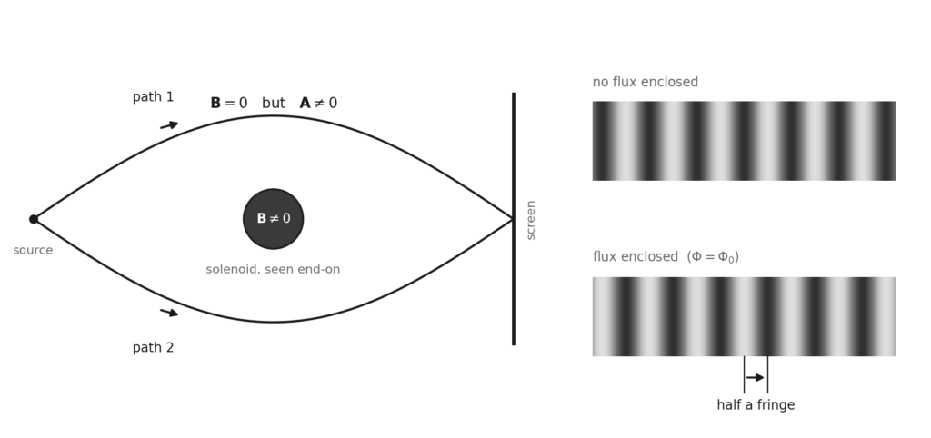
    Consider a long solenoid — a tightly wound coil carrying a steady current. Inside it there is a magnetic field. Outside it, if the coil is long enough, there is essentially none: the field is confined to the interior.

    The vector potential is a different matter. Outside the solenoid, where B vanishes, A does not. It circulates around the coil, falling off with distance but never reaching zero.

    Classically this is of no consequence whatsoever. A charged particle passing outside the solenoid experiences no magnetic field, therefore no magnetic force, therefore nothing at all. The non-zero A in that region is exactly the sort of thing one expects of a gauge-dependent bookkeeping quantity: present in the mathematics, absent from the physics.

    A classical counterpart of this geometry does exist, and is worth noting in passing. If the solenoid is driven with an alternating current, a conducting loop encircling it — but never entering it — develops a measurable electromotive force, even though the magnetic field along the loop is negligible. Faraday’s law in integral form accounts for this without difficulty, since it depends on the flux threading the circuit rather than on the field at the conductor. Rousseaux and co-workers, who studied the configuration theoretically and experimentally in 2008, named it the Maxwell–Lodge effect after an 1889 paper of Oliver Lodge, and argued that it is best understood in terms of the vector potential.

    Two differences matter. The classical effect requires the current to vary in time; with a steady current there is no electromotive force and nothing to measure. And the field outside a real solenoid is small rather than exactly zero — a gap that would take decades to close for the quantum case.

    What Yakir Aharonov and David Bohm proposed, in a paper published in Physical Review under the title Significance of Electromagnetic Potentials in the Quantum Theory, was that in quantum mechanics this is not true. An electron travelling through a region where the fields are rigorously zero is nonetheless affected by the potential, in a way that produces an observable consequence.

    Why the potentials, and not the fields

    The reason is structural, and it predates the effect by three decades. When electromagnetism is coupled to quantum mechanics, the fields do not appear in the equations at all. The potentials do.

    The coupling is introduced by the minimal substitution: in the Hamiltonian of a particle of charge q, the momentum is replaced by the canonical momentum, and the scalar potential is added to the energy.

    𝐩→𝐩−q𝐀,E→E−qφ\mathbf{p} \rightarrow \mathbf{p} – q\mathbf{A}, \qquad E \rightarrow E – q\varphi

    Written out, this is the operator that governs the evolution of the wavefunction:

    iℏ∂ψ∂t=[12m(−iℏ∇−q𝐀)2+qφ]ψi\hbar\frac{\partial \psi}{\partial t} = \left[\frac{1}{2m}\left(-i\hbar\nabla – q\mathbf{A}\right)^2 + q\varphi\right]\psi

    There is no way to write this in terms of E and B. The Schrödinger equation for a charged particle is a statement about φ and A, and always was — a fact that attracted little comment for as long as everything it predicted could also be obtained from the fields.

    Gauge invariance survives because a change of gauge multiplies the wavefunction by a position-dependent phase, which leaves every probability unchanged. But a phase that cancels in the modulus need not cancel between two interfering paths — and that is the whole of the effect.

    How you would see it

    The prediction concerns interference, so it is worth a sentence on what that means here.

    An electron beam split into two paths and recombined produces a pattern of alternating light and dark bands — fringes — because the electron behaves as a wave, and the two halves of that wave arrive either in step or out of step depending on the difference in what they have encountered along the way. Shift the relative timing of the two halves, and the whole pattern slides sideways. The size of that shift is a measurement.

    Now run one path on each side of the solenoid. Neither electron ever enters a region with a magnetic field. But the two paths, taken together, enclose the solenoid — and the phase difference between them is

    Δθ=qℏ∮𝐀⋅dℓ=qΦℏ\Delta\theta = \frac{q}{\hbar}\oint \mathbf{A}\cdot d\boldsymbol{\ell} = \frac{q\Phi}{\hbar}

    where the integral runs around the closed loop formed by the two paths, and Φ is the magnetic flux threading it. The fringes shift, by an amount fixed by the flux inside a region the electrons never visited.

    The part that is easy to state wrongly

    It is tempting to summarise this as “the vector potential is physically real after all.” That is too quick, and the precise version is more interesting.

    A is still not gauge-invariant. Change gauge and its value at any given point changes, exactly as before. What is gauge-invariant is the integral around a closed loop, because the extra term introduced by a gauge transformation is a gradient, and the integral of a gradient around any closed path vanishes identically:

    ∮∇χ⋅dℓ=0\oint \nabla\chi \cdot d\boldsymbol{\ell} = 0

    So the observable is not A at a point. It is the loop integral — a global quantity, belonging to the path as a whole rather than to any location on it.

    This has a consequence that is easy to miss. Whether the loop integral can be non-zero, in a region where the field vanishes, depends on the shape of the region. The solenoid geometry works because the electron paths enclose something they cannot enter: the accessible region has a hole in it. Given a region without such a hole — one in which every loop can be shrunk continuously to a point — a vanishing field forces the loop integral to vanish too, no matter how large A happens to be locally.

    The requirement that the solenoid be long, which reads at first like an engineering detail, is doing exactly this work. It is what makes the exterior region topologically non-trivial.

    1949

    There is an earlier paper.

    In 1949, Werner Ehrenberg and Raymond Siday published in the Proceedings of the Physical Society a study of the refractive index in electron optics which discusses a substantially equivalent effect — a decade before Aharonov and Bohm, in a journal nobody would have thought to overlook.

    It went essentially unnoticed. The result was framed as a technical point within electron optics rather than as a statement about the status of the potentials, and it reached an audience of instrument specialists rather than of physicists interested in foundations. The effect is now occasionally called Ehrenberg–Siday–Aharonov–Bohm, which is accurate and which almost nobody says.

    The pattern is the same one that swallowed Lorenz’s name, with a different mechanism. There the correct attribution lost to a more famous near-homophone. Here it lost to framing: the same physics, presented as a correction to a specialist calculation instead of as a challenge to a foundational assumption, simply did not register.

    Closing the last gap

    The prediction was contested for years, and the objection was a fair one. Real solenoids are finite. A small amount of magnetic field always leaks into the region the electrons traverse, and a sceptic could maintain that the observed shift was caused by that leakage rather than by the potential in a genuinely field-free region.

    Settling it took until the 1980s, and the work of Akira Tonomura and his collaborators at Hitachi. Electron holography experiments in 1982 established the shift. The decisive experiment came in 1986.

    They built a toroidal magnet roughly six micrometres across — a doughnut, so that the field lines close on themselves inside it with no ends to leak from — and then covered the whole thing in a superconducting shell. A superconductor expels magnetic field from its interior, the Meissner effect, so the shell acted as a barrier that no field line could cross. The magnetic field was not merely small outside the torus. It was excluded, by a mechanism independent of the geometry.

    The observed fringe shift was exactly half a fringe — the value required by the quantisation of magnetic flux in a superconductor, in units of

    Φ0=h2e≈2.07×10⁻¹⁵ Wb\Phi_0 = \frac{h}{2e} \approx 2.07 \times 10^{-15}\ \mathrm{Wb}

    Not approximately half. The number the theory demanded, produced by a system in which the alternative explanation had been physically eliminated.

    What changed

    The classical position was that the fields carry the physics and the potentials carry the bookkeeping. After 1986 that cannot be maintained. There is an experiment in which the fields are zero everywhere the particle goes, and something happens anyway.

    What replaced it is not the opposite claim. A is not an ordinary field with a definite value at each point; it remains gauge-dependent, and any description that treats its pointwise value as measurable is wrong. What the experiments establish is narrower and stranger: that there exists a gauge-invariant quantity built from the potentials, not reducible to the fields, which is not local — it belongs to a closed path rather than to a place — and which nature is demonstrably sensitive to.

    The potentials turned out not to be scaffolding. They turned out to be carrying something the field description had no way to express.


    Sources

    • W. Ehrenberg and R. E. Siday, “The Refractive Index in Electron Optics and the Principles of Dynamics,” Proc. Phys. Soc. London, vol. B62, p. 8, 1949.
    • Y. Aharonov and D. Bohm, “Significance of Electromagnetic Potentials in the Quantum Theory,” Phys. Rev., vol. 115, pp. 485–491, 1959.
    • A. Tonomura et al., “Observation of Aharonov-Bohm Effect by Electron Holography,” Phys. Rev. Lett., vol. 48, pp. 1443–1446, 1982.
    • A. Tonomura et al., “Evidence for Aharonov-Bohm Effect with Magnetic Field Completely Shielded from Electron Wave,” Phys. Rev. Lett., vol. 56, pp. 792–795, 1986.
    • N. Osakabe et al., “Experimental Confirmation of Aharonov-Bohm Effect Using a Toroidal Magnetic Field Confined by a Superconductor,” Phys. Rev. A, vol. 34, pp. 815–822, 1986.
    • G. Rousseaux, R. Kofman, and O. Minazzoli, “The Maxwell-Lodge effect: significance of electromagnetic potentials in the classical theory,” Eur. Phys. J. D, vol. 49, pp. 249–256, 2008.
  • Heaviside’s Other Equations

    Oliver Heaviside is remembered, when he is remembered at all, as the man who compressed Maxwell’s twenty equations into four. It is a reputation for tidying up: taking someone else’s theory and putting it in order.

    In 1893, in a short piece in The Electrician, he did something else entirely. He proposed that gravitation might obey equations of the same form as electromagnetism — and worked out some of what would follow if it did.

    The analogy

    The starting point is a resemblance anyone can see. Newton’s law of gravitation and Coulomb’s law of electrostatics have the same shape: an inverse-square force, proportional to the product of two quantities, one attracting masses and the other charges. Mass plays the part of charge.

    The resemblance had been noticed for a century and a half and had led nowhere in particular. What Heaviside asked was different. Electrostatics is only the static corner of electromagnetism; the full theory has a magnetic field, and disturbances that propagate. If gravity matches the corner, does it match the rest?

    Suppose it does. Then three things follow immediately, and each of them was, in 1893, a startling claim.

    There would have to be a gravitational counterpart of the magnetic field — a second field, produced not by mass at rest but by mass in motion, acting on other moving masses in a way that has no place in Newton’s theory. Heaviside had no name for it; the modern term is gravitomagnetism.

    Gravitational disturbances would have to propagate at a finite speed — and, if the analogy holds all the way, at the speed of light. In Newtonian gravity the force is instantaneous everywhere, and every attempt to give it a delay had run into trouble.

    And there would have to be a gravitational Poynting vector: a definite statement about where gravitational energy flows and at what rate. Heaviside wrote it down.

    What he did not claim

    What makes the paper interesting to read now is its restraint.

    Heaviside does not present this as a theory of gravitation. He presents it as a question about an analogy, followed by its consequences. And when he arrives at the gravitational energy flux, he admits that he does not understand what that energy actually is — the same admission Maxwell had made about the electromagnetic field, and for the same reason. The formalism produces a quantity that behaves like an energy flux. Whether something is really flowing, and if so what, the formalism does not say.

    This is worth dwelling on, because it is precisely the discipline that separates a useful analogy from a crank one. Heaviside had a construction that reproduced Newtonian gravity in the static limit and predicted new effects outside it. He could have argued that the new effects were therefore real. He argued instead that they would be real if the analogy held, and that whether it held was an open question he was not in a position to settle.

    Twenty-two years early, and on the wrong foundation

    Einstein completed General Relativity in 1915. Take the full theory, assume the gravitational field is weak and the velocities small, and linearise: what comes out is a set of equations formally very close to Maxwell’s, with a gravitoelectric field reproducing Newtonian gravity and a gravitomagnetic field generated by moving mass. This is the modern subject of gravitoelectromagnetism, and it is standard, uncontroversial physics — a limiting case of General Relativity, not an alternative to it.

    Heaviside got there in form, twenty-two years earlier, from an analogy.

    The word form is carrying weight. What Einstein’s theory says is that gravity is the curvature of spacetime, and the Maxwell-like equations emerge as an approximation valid when curvature is small. Heaviside had no spacetime, no curvature, and no principle from which his equations followed; he had a resemblance and the nerve to push it. The equations look alike. What is underneath them does not.

    Which is why the right description is not that Heaviside anticipated General Relativity. He anticipated one of its approximations, without the theory it approximates.

    The measurement

    The gravitomagnetic effect is not a formal curiosity. It is real, it is small, and it has been measured.

    A rotating mass drags the inertial frames around it — the Lense–Thirring effect, worked out in 1918. A gyroscope in orbit around the Earth should therefore precess, by a tiny amount, in the direction of the Earth’s rotation. Gravity Probe B was built to detect it: four cryogenic gyroscopes in polar orbit, launched in April 2004, collecting data from August 2004 to August 2005, with the final analysis published in 2011 after five further years of work.

    The frame-dragging drift came out at −37.2 ± 7.2 milliarcseconds per year, against a General Relativity prediction of −39.2. A milliarcsecond is about five billionths of a radian; the effect is roughly one part in a hundred and eighty of the much larger geodetic precession measured alongside it.

    It is worth being exact about what this confirms. It confirms General Relativity, whose prediction it matches. It does not confirm Heaviside’s 1893 equations, which are not the theory that predicted the number. What it establishes is that the kind of effect Heaviside reasoned his way to — a gravitational field generated by rotation, with no Newtonian counterpart — is a real feature of the world.

    What the episode is good for

    There is a version of this story that overclaims, and it is easy to write: the self-taught outsider who saw further than the establishment, whose ideas were confirmed a century later. Heaviside’s biography supports the telling — he worked outside the institutions and spent much of his life short of money — and it would be nearly true.

    Nearly true is the problem. He did not have General Relativity. His equations rest on nothing except an analogy, and analogies of that kind fail at least as often as they succeed — the same period produced mechanical models of the ether that led nowhere at all.

    The accurate version is more useful anyway. A structural resemblance between two theories is a legitimate thing to follow, and following it can put you in the right neighbourhood decades ahead of the physics that justifies being there. It does not put you in the right house. Heaviside knew the difference, which is why he wrote down what would follow if the analogy held, and stopped.

    That is a harder discipline than it sounds, and it is the reason the 1893 paper still reads well.


    Sources

    • O. Heaviside, “A Gravitational and Electromagnetic Analogy,” The Electrician, vol. 31, pp. 281–282 and 359, 1893.
    • J. Lense and H. Thirring, “Über den Einfluss der Eigenrotation der Zentralkörper auf die Bewegung der Planeten und Monde,” Phys. Z., vol. 19, pp. 156–163, 1918.
    • B. Mashhoon, “Gravitoelectromagnetism: A Brief Review,” arXiv:gr-qc/0311030.
    • C. W. F. Everitt et al., “Gravity Probe B: Final Results of a Space Experiment to Test General Relativity,” Phys. Rev. Lett., vol. 106, 221101, 2011.
  • Lorenz, Not Lorentz

    There is a condition, written down in 1867, that every student of electromagnetism meets sooner or later. It relates the two potentials of the electromagnetic field, and it is the reason those potentials can be made to propagate causally, at the speed of light, rather than adjusting themselves instantaneously across all of space.

    ∇⋅𝐀+1c2∂φ∂t=0\nabla \cdot \mathbf{A} + \frac{1}{c^2}\frac{\partial \varphi}{\partial t} = 0

    It is named after the man who published it. Almost everyone attributes it to somebody else.

    What a gauge is

    Readers who already work with gauge freedom can skip to the next section. For everyone else, the idea is worth setting out plainly, because the whole story turns on it.

    Electromagnetism can be described in two ways. One uses the fields directly — the electric field E and the magnetic field B, the things that push on a charge and that an instrument can measure. The other uses potentials: a scalar φ and a vector A, from which the fields are obtained by differentiation.

    The awkward fact about the second description is that it is not unique. Given any charge and current distribution, there is no single correct pair (φ, A). There are infinitely many, and they all describe exactly the same physical situation. Take any sufficiently smooth function χ of position and time, and transform:

    𝐀→𝐀+∇χ,φ→φ−∂χ∂t\mathbf{A} \rightarrow \mathbf{A} + \nabla\chi, \qquad \varphi \rightarrow \varphi – \frac{\partial \chi}{\partial t}

    The potentials change. The fields do not. Every measurable consequence is identical.

    The closest everyday parallel is the choice of a zero for height. To work out the potential energy of a book on a shelf, you have to decide where you are measuring from — the floor, the ground outside, sea level, the centre of the Earth. Each choice gives a different number, and none of them is the right one. But the difference in energy between the shelf and the floor comes out the same no matter which you pick, and that difference is the thing you can actually measure when the book falls. The zero is a convention. The drop is physics.

    Gauge freedom is the same situation, with a much larger space of conventions available. Choosing a gauge means picking one member of the family and agreeing to work with it. A quantity is called observable when it comes out the same regardless of that choice — and only observables can correspond to something an experiment could detect. A quantity that changes when you change gauge is an artefact of the bookkeeping, however useful it may be along the way.

    The condition at the top of this page is one such choice. It does not add physics. It fixes a convention — and, as it turns out, a particularly good one.

    Copenhagen, 1867

    Ludvig Valentin Lorenz was born in Helsingør in 1829 and became the first Danish theoretical physicist to gain an international reputation. In 1867 he published, in the Philosophical Magazine, a paper with the title On the Identity of the Vibrations of Light with Electrical Currents.

    He was working from Maxwell’s theory, which he had read closely. What he obtained were general integral solutions of the field equations in which the finite speed of light is built in explicitly: the potential at a point now depends on what the sources were doing earlier, at a time separated by exactly the light-travel delay. These are the retarded potentials.

    φ(𝐫,t)=14πε0∫ρ(𝐫′,t′)|𝐫−𝐫′|dV′𝐀(𝐫,t)=μ04π∫𝐉(𝐫′,t′)|𝐫−𝐫′|dV′\varphi(\mathbf{r},t) = \frac{1}{4\pi\varepsilon_0}\int \frac{\rho(\mathbf{r}’,t’)}{|\mathbf{r}-\mathbf{r}’|}\,dV’ \qquad\qquad \mathbf{A}(\mathbf{r},t) = \frac{\mu_0}{4\pi}\int \frac{\mathbf{J}(\mathbf{r}’,t’)}{|\mathbf{r}-\mathbf{r}’|}\,dV’
    t′=t−|𝐫−𝐫′|ct’ = t – \frac{|\mathbf{r}-\mathbf{r}’|}{c}

    The gauge condition falls out of this construction rather than being imposed on it. That is the point that gets lost when it is described as one convenient choice among several: it is the choice under which the potentials themselves respect causality, propagating outward at c like everything else in the theory.

    Maxwell, for his part, did not receive the work warmly.

    Göttingen, 1861

    There is an earlier thread, reported by the historian Edmund Whittaker in his History of the Theories of Aether and Electricity. Bernhard Riemann had discussed substantially the same condition in lectures in 1861 — six years before Lorenz, and never in print.

    This is a familiar shape in the history of science, and it cuts in an unexpected direction here. It does not diminish Lorenz’s claim; it strengthens it. Priority in science attaches to publication, not to private insight, precisely because publication is what makes an idea available to everyone else. Riemann thought of it. Lorenz put it where it could be used.

    Which makes what happened next harder to excuse.

    The other Lorentz

    Hendrik Antoon Lorentz was Dutch, born in 1853, and a physicist of the first rank in his own right: the transformations that bear his name, the electron theory of matter, the Nobel Prize in 1902 shared with Zeeman. He is one of the figures without whom twentieth-century physics does not happen.

    He also had nothing to do with the gauge condition. When Lorenz published it in 1867, Lorentz was fourteen years old.

    The attribution nonetheless drifted to him, and stuck, for two reasons that reinforce each other. The first is simply that the names sound alike and differ by one letter. The second is more interesting: the Lorenz condition happens to be Lorentz-invariant. It is compatible with special relativity, unchanged in form under a change of inertial frame — which is exactly what one would expect of something Lorentz had produced, and which is in fact a coincidence of a Danish physicist writing four decades before relativity existed.

    An error that plausible is very hard to dislodge. It appears in serious scientific literature and in reference texts, Feynman’s among them, and it has needed a small specialist literature of its own to document: van Bladel in 1991, Nevels and Shin in 2001, and the historical review by Jackson and Okun in the same year.

    It is a clean case study in how attribution actually works. A name does not win in collective memory by being correct. It wins by being familiar, and by fitting the story the reader already expects.

    Why the choice matters

    Gauge freedom means no choice is more true than another. It does not mean every choice is equally convenient, and the differences are substantial.

    The Coulomb gauge sets the divergence of A to zero. It reduces the equation for the scalar potential to an ordinary Poisson equation, which makes electrostatic problems straightforward — at the cost that φ then appears to respond instantaneously to a change in the charge distribution anywhere in the universe. Nothing observable propagates faster than light; the apparent instantaneity is confined to the potential and cancels in the fields. But you have to know that, and keep track of it.

    The Lorenz gauge does not have that feature. Both potentials satisfy wave equations, both propagate at c, and causality is manifest in the formalism rather than something one has to argue for afterwards.

    If gauges are lenses, this is the sense in which they differ: not that one shows more of the object, but that each is ground for a different kind of work. The Coulomb gauge is the right lens for a static problem. The Lorenz gauge is the right lens for anything that has to travel.

    It is worth calling it by the name of the man who published it.


    Sources

    • L. V. Lorenz, “On the Identity of the Vibrations of Light with Electrical Currents,” Phil. Mag., series 4, vol. 34, pp. 287–301, 1867.
    • E. T. Whittaker, A History of the Theories of Aether and Electricity, vol. 1. London: Nelson, 1910; rev. 1951.
    • J. Van Bladel, “Lorenz or Lorentz?,” IEEE Antennas and Propagation Magazine, vol. 33, no. 2, p. 69, 1991.
    • R. Nevels and Chang-Seok Shin, “Lorenz, Lorentz, and the Gauge,” IEEE Antennas and Propagation Magazine, vol. 43, no. 3, pp. 70–71, 2001.
    • J. D. Jackson and L. B. Okun, “Historical Roots of Gauge Invariance,” Rev. Mod. Phys., vol. 73, pp. 663–680, 2001.
  • Did Maxwell Write in Quaternions?

    On the afternoon of 16 October 1843, walking with his wife along the towpath of the Royal Canal in Dublin, William Rowan Hamilton found the thing he had been looking for over several years: a four-dimensional number system, closed under multiplication, obeying the rule i² = j² = k² = ijk = −1. He carved it into the stone of Broom Bridge on the spot. A plaque there still records the moment.

    Twenty-one years later, Maxwell read his dynamical theory of the electromagnetic field to the Royal Society. It is often said that he wrote that theory in Hamilton’s algebra, and that Oliver Heaviside later tore the quaternion structure out and replaced it with the vector calculus every student now learns. The story is appealing: a richer mathematics, discarded for convenience, with something lost in the exchange.

    It is also, in the form usually told, wrong — and the accurate version is more interesting.

    What the 1865 paper actually contains

    The paper has a well-documented history. Maxwell sent it to the Royal Society on 27 October 1864; it was read on 8 December of that year; it went to William Thomson for review before Christmas and to George Gabriel Stokes the following March; the Committee of Papers approved it on 15 June 1865 and it went to the printers the next day. It appeared as A Dynamical Theory of the Electromagnetic Field in Philosophical Transactions, volume 155, pages 459–512. The original manuscript — 84 pages in Maxwell’s hand — is still in the Society’s archives.

    Open it, and there are no quaternions.

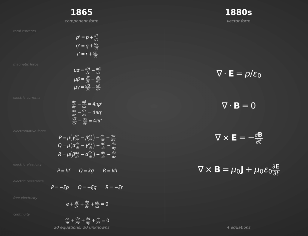
    What there is instead is twenty equations in twenty unknowns, written out component by component in Cartesian coordinates. Faraday’s law occupies three separate lines, one each for the components Maxwell calls P, Q and R. The Ampère–Maxwell law occupies three more, for α, β and γ. Derivatives appear one axis at a time: d/dx, then d/dy, then d/dz. There is no Hamiltonian product anywhere, no scalar-plus-vector object, nothing that requires the algebra carved on Broom Bridge.

    The count itself is the giveaway. Twenty equations are needed precisely because each vector relation has to be written three times over. With a compact formalism — any compact formalism — four will do, which is exactly what Heaviside would later demonstrate.

    This does not mean Maxwell lacked the vector idea. He plainly had it. The quantities we now write as single bold letters are there in his text as triples of separate symbols: the electric field as (P, Q, R), the magnetic induction as μ(α, β, γ), the vector potential as (F, G, H). He knew these belonged together. He had no notation in working order that would let him say so in one line.

    Worth noting in passing: the twenty equations also include Ohm’s law, the force on a moving charge, and the continuity of electric charge — relations nobody today calls one of Maxwell’s equations. The set we now teach under his name was not only re-notated after his death. It was reselected.

    1870, and the Treatise

    Maxwell’s interest in quaternions was real, and it came later.

    In November 1870 he wrote a manuscript specifically on the application of quaternions to electromagnetism, and he corresponded on the subject with Peter Guthrie Tait — Hamilton’s collaborator, and the most committed advocate the algebra had in Britain. In the Treatise on Electricity and Magnetism of 1873, a more condensed quaternion notation appears for the general field equations, in the second volume.

    So the honest sequence is: no quaternions in 1865, a manuscript on the question in 1870, condensed quaternion notation in the 1873 Treatise. The mythology compresses this into a single origin that never existed.

    Even in the Treatise, the use is limited. On the analysis of the historian André Waser, Maxwell employed quaternions as an expository and symbolic language rather than as an operational tool — a way of displaying the structure of a result, not a machinery he calculated in daily. Whether that judgement holds under a page-by-page reading of the relevant chapter is a question worth putting to the original text rather than taking on authority, and one I intend to return to.

    The most defensible summary is this: Maxwell was genuinely interested in quaternions, adopted them partially, and never brought their systematic use in electromagnetism to completion. He introduced the tool into the subject. He did not build with it.

    Heaviside, Gibbs, and the four equations

    Maxwell died in 1879, at forty-eight.

    The reformulation came afterwards. Through the 1880s, Oliver Heaviside — self-taught, working outside the institutions, and in financial difficulty for much of his life — developed a vector calculus and rewrote the twenty equations into the four with divergence and curl that are now universal. Josiah Willard Gibbs arrived at substantially the same system independently at Yale.

    The chronology matters for the story. There was no confrontation between Maxwell and Heaviside over notation, and Maxwell did not live to see his own formulation set aside. Whatever was decided about quaternions in electromagnetism was decided by other people, in a debate he was not present for.

    Why the vector form won is not mysterious. It was fitted to the problems that mattered at the moment it appeared. The rising technology of the period was radio, and radio is dominated by transverse waves in free space, where the vector calculus is exactly adequate and quaternions are overhead. Heaviside’s system was leaner for the work in front of it, and it worked — unambiguously, for well over a century, underwriting almost everything electrical that followed.

    The war of the vectors

    The quaternionists did not concede quietly. Through the 1890s, in the pages of Nature and elsewhere, Tait fought a long rearguard action against Gibbs and Heaviside, defending Hamilton’s algebra as the proper language of physics against what he regarded as a mutilation of it.

    He lost, comprehensively. By the turn of the century the vector notation was standard in physics teaching, and quaternions had been pushed to the margins of the curriculum, where they remained until computer graphics and spacecraft attitude control found a use for them in representing rotations — a role that has nothing to do with the one Tait was arguing for.

    The point worth holding onto is who was arguing. The defence of quaternions in electromagnetism was mounted by Tait, not by Maxwell, and it was mounted after Maxwell was dead.

    Abandoned, not refuted

    Nothing in this history involves anyone showing that the quaternion approach to electromagnetism was wrong. No calculation failed, no prediction came out false, no inconsistency was exposed. The programme was not defeated. It was set down, by a man who had other things to finish, and never picked up again — because within a few years something more convenient had arrived for the problems then at hand.

    That is a weaker claim than the mythological version, and a more durable one. It also leaves a question standing that the mythological version answers too quickly. If a formalism is put aside because it is heavier than the problems of the day require, the natural thing to ask is what happens at problems it was never tested against — and whether the reduction that made the vector calculus so efficient for transverse waves in free space discarded anything along with the notation.

    That question does not answer itself, and it is not answered here. But it is a real question, and it is worth keeping the history straight in order to ask it properly.


    Sources

    • J. C. Maxwell, “A Dynamical Theory of the Electromagnetic Field,” Phil. Trans. R. Soc., vol. 155, pp. 459–512, 1865. Read 8 December 1864.
    • Manuscript, Royal Society Archives, PT/72/7 — received 27 October 1864.
    • J. C. Maxwell, A Treatise on Electricity and Magnetism, vol. 2. Oxford: Clarendon Press, 1873, Ch. IX.
    • A. Waser, “On the Notation of Maxwell’s Field Equations,” AW-Verlag, 2000.
    • O. Heaviside, Electromagnetic Theory, 3 vols. London: The Electrician, 1893–1912.
    • W. R. Hamilton, “On quaternions,” Proc. R. Irish Acad., vol. 3, pp. 1–16, 1847.
    • M. Longair, “A commentary on Maxwell (1865),” Phil. Trans. R. Soc. A, vol. 373, 20140473, 2015.