What the causal solution of Maxwell’s equations actually says
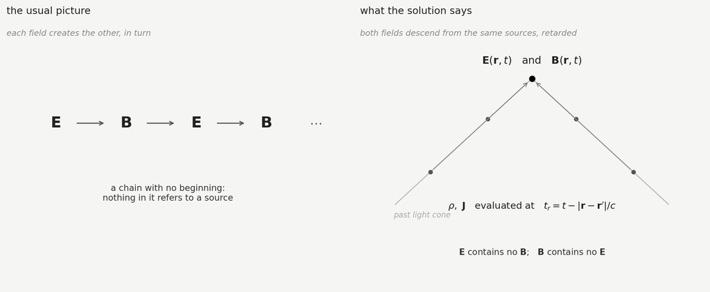
Almost every introduction to electromagnetic waves tells the same story. A changing electric field produces a magnetic field; that magnetic field, also changing, produces an electric field; and the two, taking turns, hand energy back and forth as the disturbance propagates away. It is a vivid picture, it appears in textbooks and lecture courses everywhere, and it makes the wave feel like something that sustains itself once launched.
There is a way of writing the solution of Maxwell’s equations in which that picture does not appear at all. In it, the electric field at a point contains no reference to the magnetic field anywhere, and the magnetic field contains no reference to the electric one. Both are written entirely in terms of charges and currents, evaluated at earlier times. Nothing takes turns with anything.
The equations are usually named after Oleg Jefimenko, who published them in 1966. Whether the picture they displace is wrong, or merely not forced, turns out to be a more delicate question than either side of the argument usually admits — and the delicate part is where this article ends up.
What the causal solution looks like
Maxwell’s equations in differential form relate fields and sources at a single instant. The curl equations in particular put a time derivative of one field on one side and the other field on the other side, both evaluated now:
Read as a statement of what causes what, this is already strange. The two sides are simultaneous. Whatever relation holds between them, it is not one in which the right-hand side has had time to bring the left-hand side about, because no time has passed at all. Jefimenko put the point bluntly: since each of these equations connects quantities simultaneous in time, none of them can represent a causal relation.
The solution of the same equations, for an arbitrary distribution of charge and current, can be written so that the time structure is explicit. Two pieces of shorthand keep it readable: R for the vector from a source point to the point of observation, and a dot for a time derivative. The retarded time follows from the first:
That is, the moment early enough that a signal leaving the source point then, travelling at c, arrives at the observation point now. Every source quantity in what follows — ρ, J, and their time derivatives — is evaluated at that earlier moment, never at the observation time. With that understood, the electric field is
and the magnetic field
Two features of these expressions do the work, and both are visible without evaluating a single integral.
The first is that the right-hand sides are in the past. Not simultaneous, not implicitly retarded, but explicitly evaluated at an earlier instant fixed by the light travel time. Whatever the sources were doing then determines what the fields are here now.
The second is what is missing. The expression for E contains ρ and J and their time derivatives. It does not contain B. The expression for B contains J and its time derivative. It does not contain E. Neither field appears in the other’s formula, at any time, retarded or otherwise. Jefimenko’s own conclusion follows directly: the electromagnetic field is a dual entity, always having an electric and a magnetic component, simultaneously created by their common sources — time-varying charges and currents.
Why they are locked together in the far field
There is an obvious objection, and it is worth meeting head-on. Far from any source, the two fields are not merely correlated but rigidly tied: the magnetic field is perpendicular to the electric one and to the direction of propagation, with magnitudes in the fixed ratio
That is about as tight a relationship as two quantities can have. If neither field has anything to do with the other, why do they march in lockstep?
The answer is visible in the expressions themselves, once one asks which terms survive at large distance. Of the three contributions to E, the first falls off as 1/R² and is negligible far away; the two carrying time derivatives of the sources fall only as 1/R and are what remains. Charge conservation then does something specific: the longitudinal part of the current-derivative term cancels exactly against the charge-derivative term, and what is left is the transverse part of the current derivative alone. In the expression for B, the surviving 1/R term is that same current derivative, crossed with R̂ — which selects precisely the same transverse quantity.
Written out, with J̇⊥ for the part of the current derivative perpendicular to the line of sight, the two radiation fields are:
So in the radiation zone both fields reduce to integrals over one and the same thing: the transverse acceleration of charge at the retarded time. One of them carries an extra cross product with the line of sight, and that is the entire difference between them. The fixed ratio and the mutual perpendicularity follow from that by algebra, not by any influence passing between them.
This is a common-cause correlation, and the distinction is not a quibble. Two quantities descending from the same ancestor can be rigidly related without either producing the other — and the structure here shows exactly that pattern, because the lockstep holds only where both expressions collapse onto the shared term. Closer in, where the 1/R² contributions are still present, the ratio of the field magnitudes is not c, the two are not in phase, and the neat orthogonality fails. Any mechanism by which one field genuinely generated the other would have to operate everywhere, not only in the region where the two formulas happen to reduce to the same integral.
The far-field relation, in other words, is the strongest-looking evidence for the mutual-induction picture, and on inspection it is evidence against it.
Where they come from
Nothing new is being introduced. These are Maxwell’s equations, solved, and the route is short.
Start from the retarded potentials in Lorenz gauge — the same objects, and the same gauge condition, discussed elsewhere on this site:
Then substitute the definitions of the fields in terms of the potentials, and differentiate under the integral sign. The derivatives act on the retarded time as well as on the explicit distance dependence, which is where the extra terms in 1/R and 1/R² come from. What emerges is the pair above.
This matters for how much weight the result can carry. Jefimenko’s equations are not an alternative theory, a modification, or a reinterpretation. They are the general solution of the standard equations, written in one particular way. Anything true of them is true of Maxwell’s electrodynamics; the question is only what becomes visible in this form that was hidden in the other.
Who wrote them first
The attribution is tangled in a way that will be familiar to anyone who has followed the Lorenz and Ehrenberg–Siday cases discussed elsewhere here.
David Griffiths, whose textbook is where most physicists meet these expressions, is careful about it: the earliest explicit statement of which he is aware was Jefimenko’s, in 1966. Kirk McDonald has pointed out that time-domain expressions of essentially this form appear four years earlier, in the second edition of Panofsky and Phillips’s Classical Electricity and Magnetism of 1962, where the electric field is written in a slightly different but entirely equivalent form. And the closely related formula for the fields of a single point charge in arbitrary motion — often called the Heaviside–Feynman formula — was published by Oliver Heaviside in 1904, then rediscovered by Feynman and presented in the Lectures in 1963, apparently without knowledge of the earlier result.
Three independent arrivals, spanning six decades, at expressions that were available in principle from the moment the retarded potentials were understood. The pattern is the one this site keeps running into: the mathematics was not the obstacle. What was missing each time was a reason to write the solution in that particular form, and an audience for whom the form mattered.
Jefimenko’s contribution, on the evidence, was less the derivation than the insistence on what it meant. Panofsky and Phillips wrote the expressions and moved on. Jefimenko spent decades arguing about them.
What this does not settle
Here the argument needs slowing down, because the strong version of the claim is repeated more often than it is examined, and it does not survive contact with two facts.
Retardation was chosen, not derived
The retarded solution is not the only solution of Maxwell’s equations. There is also an advanced one, identical in form except that the sources are evaluated at
— that is, in the future. It satisfies the same equations exactly as well. The full general solution is any combination of the two, plus a source-free solution of the homogeneous equation.
Choosing the retarded solution alone is a physical input, made on the grounds that fields should propagate outward from sources rather than converge inward from infinity. It is a boundary condition, and a well-motivated one, but it is not a consequence of Maxwell’s equations. So the causal structure that Jefimenko’s form displays so clearly was, in a precise sense, put in by hand at the moment the retarded Green’s function was selected.
This does not make the equations wrong or the argument empty. It relocates it. The equations do not prove that sources cause fields rather than fields causing each other; they show that once the ordinary radiation boundary condition is imposed, the solution can be written entirely in terms of sources, with no field-on-field dependence anywhere. That is a genuine structural fact about the theory, and it is not what the mutual-induction story leads one to expect.
The equations describe fields produced by given sources, and nothing else
The second limitation is stated in the equations’ own preamble and is easy to read past. They give the fields produced by an assigned distribution of charge and current, on the assumption that there is no electromagnetic field present other than the one those sources produce.
A plane wave crossing empty space with no sources anywhere is a perfectly good solution of Maxwell’s equations, and Jefimenko’s expressions have nothing to say about it: with ρ and J set to zero, both integrals vanish, and one is left with the source-free solution that had to be added separately. The same applies to a field in a resonant cavity long after whatever excited it has been switched off.
So the claim cannot be that no electromagnetic field ever exists without sources. It is narrower: that the fields of a given source distribution are determined by that distribution alone, with the two components arising together rather than one generating the other.
The dispute is live
None of this is settled interpretation. Jefimenko’s causal reading was challenged directly in the pages of the American Journal of Physics — Rohrlich argued in 2002 that the Coulomb field’s causal status does not work the way Jefimenko’s programme requires, Jefimenko replied in the same volume, and Rohrlich replied again. Reasonable physicists disagree about how much metaphysical weight a choice of Green’s function can bear.
What is not in dispute is the mathematics. Everyone agrees the expressions are correct solutions of Maxwell’s equations, and everyone can see that E does not appear in the formula for B.
The same point, seen in another algebra
The argument above was made by comparing two expressions and observing what each one lacks. There is a formalism in which the observation needs no comparison, because the two fields are not two objects to begin with.
In the biquaternion formulation used throughout this site — in One Operator, Four Domains and The Fifth Equation — the potentials and the sources are each a single object, scalar part imaginary and vector part real:
Applying the operator twice gives the whole inhomogeneous system in one line, the wave equations for both potentials at once:
And applying it once to the potential gives the fields — not two expressions to be compared, but the two slots of a single result:
The vector slot carries both fields together, 2B − (2i/c)E; the scalar slot carries the Lorenz quantity b.
Written this way, the point of this article stops being an inference and becomes a feature of the notation. One does not check that E fails to appear in the formula for B, because there is no separate formula for either: there is one object, produced by one operation acting on one retarded source. That the two components arise together, from a common ancestor, is not a conclusion drawn from inspecting the solution — it is what the solution is.
The far-field relation reads the same way. If the fields are two slots of one object, the rigid tie between them at large distance is a condition on that object, not a negotiated agreement between two independent entities. The transverse structure that emerged above from cancellation between terms is, in this language, a statement about what survives in the vector slot at order 1/R.
One further remark belongs here, because it bears on what this article has been arguing. That same single application also fills the scalar slot — with the Lorenz condition, as developed at length in The Fifth Equation. The gauge condition is not an auxiliary constraint bolted on to four field equations; it arrives with them, from the same operation. That matters in the present context, because the retarded solution used throughout this article is the Lorenz-gauge one, and the causal structure everything here depends on is inseparable from that choice.
The same algebra has been developed independently outside this programme, in different conventions: Gsponer writes Maxwell’s inhomogeneous system as a single biquaternion equation for a field bivector, and takes the construction back through Paul Weiss’s quaternionic radiation theory of 1941 to Hamilton himself. The notation differs — Gaussian units, c = 1, the fields carried as a bivector rather than in the slots used here — but the structure is the same one, and readers coming from that literature will recognise it.
Nothing in this section is a new result, and no claim of one is intended: this is the same solution of the same equations, written in an algebra that happens to make one of its features conspicuous. But that is worth something on its own. A formalism in which a true statement is hard to see, and another in which it is hard to miss, are not equally good descriptions of the same physics — and which of the two is the standard one is a matter of history rather than of merit.
What survives
The useful residue is smaller than the strongest claims made for these equations, and more solid.
The mutual-induction story is a picture attached to a particular way of writing the equations, not a fact the equations assert. Written in the form above, the same theory offers no support for it at all: two fields, both descending from the same sources at the same retarded time, neither making any reference to the other.
It is worth being fair about where that picture comes from, because it is not arbitrary. In Heaviside’s local form — the differential equations as every course presents them — the curl of E genuinely is tied to the rate of change of B, and the curl of B to the rate of change of E. As a statement about constraint, that reading is correct: given one field, the other is not free. The two are rigidly linked at every point, and the local equations are exactly where one sees it.
What the local form cannot show is why they are linked. A constraint between two quantities is equally well explained by one producing the other and by both descending from a common ancestor, and nothing in the differential equations distinguishes the two — not least because, as Jefimenko pointed out, their two sides are simultaneous, so neither has had time to bring the other about. The retarded form settles what the local form leaves open: the ancestor is there, in the sources, and the constraint is what remains of it.
So the slippage is a narrow one, and easy to make. A student told that a changing E creates a B which creates an E has been handed a correct description of a constraint, relabelled as a mechanism.
Whether that mnemonic is harmless is a matter of taste, but it has a cost worth noting. It suggests that a wave, once launched, sustains itself by an internal exchange — and therefore that something about the wave is doing work to keep it going. Jefimenko’s form makes clear that nothing needs to sustain anything: the field at a distant point now is simply what the sources were doing at the retarded time, propagated outward, with no bootstrapping required.
That is a modest result. But it is the kind of modesty that follows from writing the same thing a second way and looking at what changed — which, in a subject where the standard formalism has been fixed for over a century, is one of the few remaining ways to learn something about it.
Sources
- O. D. Jefimenko, Electricity and Magnetism: An Introduction to the Theory of Electric and Magnetic Fields. New York: Appleton-Century-Crofts, 1966; 2nd ed., Star City: Electret Scientific, 1989.
- O. D. Jefimenko, Causality, Electromagnetic Induction, and Gravitation, 2nd ed. Star City: Electret Scientific, 2000, ch. 1 (source of the quoted remarks on simultaneity and on the dual nature of the field).
- W. K. H. Panofsky and M. Phillips, Classical Electricity and Magnetism, 2nd ed. Reading, MA: Addison-Wesley, 1962, sec. 14.3.
- K. T. McDonald, “The relation between expressions for time-dependent electromagnetic fields given by Jefimenko and by Panofsky and Phillips,” Am. J. Phys., vol. 65, no. 11, pp. 1074–1076, 1997.
- D. J. Griffiths and M. A. Heald, “Time-dependent generalizations of the Biot–Savart and Coulomb laws,” Am. J. Phys., vol. 59, no. 2, pp. 111–117, 1991.
- D. J. Griffiths, Introduction to Electrodynamics, 3rd ed. Upper Saddle River: Prentice Hall, 1999, pp. 427–438.
- O. Heaviside, Electromagnetic Theory, vol. 3, 1904 (point-charge field formula); R. P. Feynman, R. B. Leighton and M. Sands, The Feynman Lectures on Physics, vol. 1, 1963, sec. 28-1.
- A. Gsponer, “Derivation of the potential, field, and locally-conserved charge-current density of an arbitrarily moving point-charge,” ISRI-06-04, arXiv:physics/0612232 (biquaternion treatment of the retarded point-charge field).
- P. Weiss, “On some applications of quaternions to restricted relativity and classical radiation theory,” Proc. Roy. Irish Acad., vol. 46, pp. 129–168, 1941.
- A. Gsponer and J.-P. Hurni, “The physical heritage of Sir W. R. Hamilton,” arXiv:math-ph/0201058.
- F. Rohrlich, “Causality, the Coulomb field, and Newton’s law of gravitation,” Am. J. Phys., vol. 70, pp. 411–414, 2002; O. D. Jefimenko, comment, and F. Rohrlich, reply, Am. J. Phys., vol. 70, p. 964, 2002.
Leave a Reply