Late in the evening of 8 July 1962, local time, the streetlights failed along several strings in Oahu. Burglar alarms went off across the islands. A microwave repeater on Kauai stopped working, cutting telephone traffic between Kauai and the other islands. The input stages of ionospheric sounders failed; rectifiers in communication receivers were damaged.
The cause was 1,445 kilometres away, and 400 kilometres up.
At 09:00 UTC on 9 July, a 1.4-megaton device had been detonated above Johnston Island in the Pacific, in a test named Starfish Prime. What reached Hawaii was not blast, not heat, not fallout. It was an electromagnetic pulse — and the instruments deployed to measure it were driven off scale, which is a polite way of saying that the most important measurement of the experiment was lost at exactly the moment it mattered.
This article is about the physics of that pulse, and about how it was worked out afterwards, from a partial record, by people who had guessed wrong the first time.
Two wrong answers
By 1962 there were already models for what a nuclear detonation should do electromagnetically. Neither of them worked.
The first, associated with Hans Bethe, treated the problem as a downward-directed current: charge separation driven radially outward from the burst, with the resulting current radiating. For a burst inside dense air, close to the ground, this is roughly right — the geometry is compact and the radiation is modest. Extrapolated to 400 km, it gave an answer far too small.
The second was the magnetohydrodynamic mechanism: the expanding, highly conductive fireball excludes the geomagnetic field, pushing it aside like a bubble in a fluid, and the field’s subsequent relaxation drives currents in the ionosphere and, by induction, in long conductors on the ground. This is real physics — it does happen, and we will come back to it — but its characteristic timescale is seconds, not nanoseconds. It could not account for a fast, high-amplitude pulse.
Both models failed in the same direction. They underestimated the peak by orders of magnitude. That is worth stating plainly, because the usual account of Starfish Prime presents the EMP as a discovery, when it is more accurately described as the failure of two predictions.
What Longmire saw
The correct mechanism was identified by Conrad Longmire at Los Alamos in 1963, and published in full form much later. The essential move is to stop thinking about the fireball and start thinking about the air, tens of kilometres below it.
A fission or thermonuclear detonation emits a prompt burst of gamma rays. At 400 km altitude there is essentially nothing for them to interact with, so they stream outward in straight lines at c. Moving downward, they eventually reach air dense enough to matter — roughly between 20 and 40 km altitude, where the density is still low by sea-level standards but no longer negligible. This layer is the source region, and it is where all the interesting physics happens.
In the source region, gamma rays Compton-scatter off atomic electrons. The kinematics of Compton scattering at these energies are strongly forward-peaked: the recoil electrons are relativistic and they move, on average, in the same direction the gamma ray was going. So the gamma flux converts itself into an electron flux, propagating radially outward from the burst.
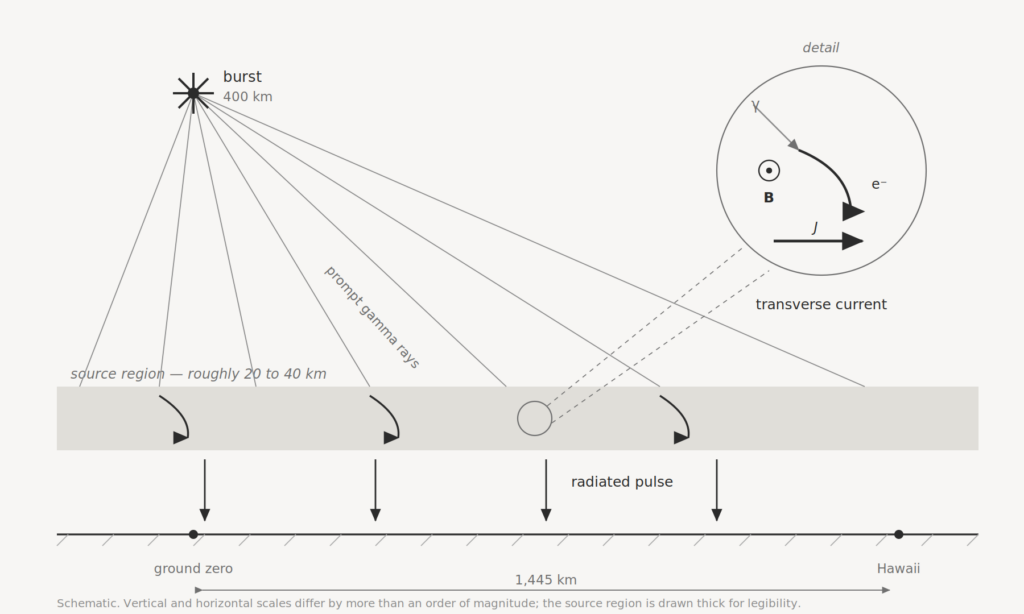
A radial current alone is a poor radiator. What makes this one efficient is the third ingredient, and it was not supplied by the weapon.
The Compton electrons are relativistic charged particles moving through the Earth’s magnetic field, and they are therefore deflected. Whether that deflection matters is a question with a numerical answer, and it is worth working out, because it is what fixes the altitude of the source region.
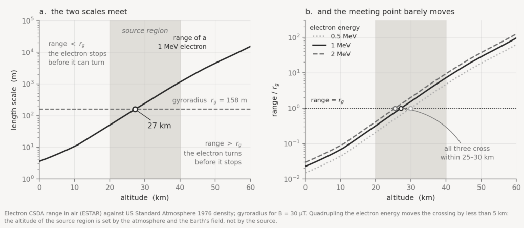
Two lengths compete. The first is the gyroradius, the scale on which the magnetic field bends the trajectory. For an electron of kinetic energy 1 MeV the momentum is 1.42 MeV/c, and in a field of 30 μT
independent of altitude, since the geomagnetic field barely changes over the first hundred kilometres. The second is the range: how far the electron travels before collisions bring it to rest. This one depends strongly on altitude, because it is a fixed mass per unit area — about 0.44 g/cm2 for a 1 MeV electron — divided by the local air density. At sea level that is 3.6 metres. At 30 km it is 245 metres.
The two cross at 27 km. Below that altitude the electron stops before the field can turn it and the deflection is a negligible correction; above it, the electron completes a substantial arc and the deflection becomes the dominant feature of the trajectory.
That crossing is remarkably insensitive to the electron energy. Quadrupling it, from 0.5 to 2 MeV, moves the crossing only from 30 km to 25.5 km — because gyroradius and range both grow with energy, and the growth largely cancels in the ratio. Which means something worth stating plainly: the altitude of the source region is set by the Earth’s atmosphere and the Earth’s magnetic field. The source has almost no say in it.
Above the crossing, then, the radial current acquires a large transverse component, perpendicular to both the propagation direction and the local field. And a transverse current sheet radiates.
That is the whole mechanism. It is textbook classical electrodynamics — accelerated charge, retarded fields, a current distribution with the right geometry — applied in a configuration nobody had considered because nobody had built one. The radiating structure is a shell of ionized air perhaps thirty kilometres thick and hundreds of kilometres across, illuminated coherently from above by a source at the speed of light. Its effective aperture is enormous, and the Earth’s own magnetic field is one of its components.
Nobody designed it. It assembled itself in a few tens of nanoseconds.
Why it is coherent, and why it saturates
Two features of the geometry deserve attention, because they are what separate this from an ordinary radiation problem.
Coherence. The gamma front travels down at c. The electromagnetic wave produced in the source region also travels at c. An observer on the ground below therefore receives contributions from a large volume of the source region very nearly in phase — the retardation almost exactly cancels the propagation delay of the driving front. The result is constructive addition over a huge radiating volume, and a rise time set not by the size of the structure but by the sharpness of the gamma pulse: nanoseconds. The spectrum is correspondingly broad, which is why the pulse coupled into everything from streetlight strings to receiver front ends.
Saturation. The same Compton electrons that carry the current also ionize the air, and ionized air conducts. The conductivity rises during the pulse and begins to short-circuit the very current that produced it: secondary electrons drift under the induced field in the direction that opposes the primary current.
The equations in this form are due to Karzas and Latter; Longmire’s review presents them with unusual economy. Working in retarded coordinates along the propagation path, and assuming the field varies far more slowly in space than in time, the whole problem collapses onto a single line of sight. What is left is one ordinary differential equation:
where JθC and Eθ are the transverse components of the Compton current density and of the field, σ the rising conductivity of the ionized air, and Z0 = 377 Ω the impedance of free space. There is a second, identical equation for the φ component; the two are linked by Bθ = −Eφ and Bφ = Eθ, which is why the free-space impedance appears here at all — it is not a fitted coefficient but μ0c, arriving on its own.
The derivative is not dE/dz but (1/r)·∂(rE)/∂r, and the difference matters: the 1/r is the wavefront spreading as it goes. The antenna is growing while it radiates.
One equation, and it contains both the source and the mechanism that extinguishes it.
The consequence is immediate. The field stops growing when the bracket vanishes,
so the pulse is capped not by how much current is produced but by how fast the medium becomes conducting. Setting the two terms equal over a path length L gives a threshold conductivity of order σ ≈ 2/(Z0L). Read that as a statement about impedance rather than about conductivity, and it says something clean: the source region shorts itself out when its sheet conductance reaches the admittance of free space. It is impedance matching, running in reverse — the same 377 Ω that governs how efficiently an antenna couples to empty space, here setting the ceiling on how large the pulse can become.
This is why the peak does not scale indefinitely, and why above a certain point additional gamma output buys nothing. The pulse is bounded by the electrodynamics of the medium, not by the source.
Three pulses, not one
Modern practice distinguishes three components, labelled E1, E2 and E3. The taxonomy is a later formalization — it is not the language of 1962 — but it is a genuine physical distinction, because the three arise from different mechanisms on timescales separated by many orders of magnitude.
E1 is the Compton–geomagnetic mechanism just described: nanosecond rise, tens of nanoseconds duration, high field amplitude, broad spectrum. It couples to anything with a dimension comparable to its wavelengths — cables, antennas, circuit traces.
E2 is the intermediate-time component, driven by scattered gamma rays and by neutron-induced reactions, extending into the microsecond–millisecond range. Its characteristics resemble a lightning strike, which is why it is the least troublesome: existing protection was designed for exactly this.
E3 is the slow one, and it is the MHD mechanism from the second failed model — not wrong, merely a different phenomenon. Timescale: seconds to minutes. It is functionally an artificial geomagnetic storm, and like a natural one it induces quasi-DC currents in very long conductors — power lines, pipelines, telegraph cables.
The clearest evidence for E3 does not come from Starfish Prime. On 22 October 1962 the Soviet Union conducted a high-altitude test over Kazakhstan, part of the series later known in the West as Project K. The yield was far smaller than Starfish — a few hundred kilotons — but the burst was over a large populated landmass at a higher geomagnetic latitude, and the ground below was crossed by long buried power lines. The induced surge started a fire in a power plant at Karaganda.
That result was not available outside the Soviet Union for three decades. It became known to Western researchers only after 1991, when Russian scientists were able to publish on the subject. It is a useful reminder of what the empirical base for this field actually consists of: a small number of experiments, unevenly instrumented, unevenly reported, conducted over about five years.
The other half: belts
The pulse was not the only thing Starfish Prime left behind, and the second effect had been predicted correctly — by someone who was not, formally, a physicist.
Nicholas Christofilos, at what is now Lawrence Livermore, had proposed in 1957 that beta electrons from the decay of fission fragments, released above the atmosphere, would be captured by the geomagnetic field. The argument rests on the adiabatic invariants of charged-particle motion: an electron on a field line spirals, mirrors near the poles where the field is strong, and drifts in longitude, so that within a few minutes an initially localized injection smears into a shell encircling the planet. Christofilos was reasoning by analogy with the radiation belts James Van Allen had just discovered with Explorer I.
The idea was tested with unusual speed. Explorer IV was instrumented by Van Allen’s group and launched on 26 July 1958. Three small devices were detonated at high altitude over the South Atlantic on 27 August, 30 August and 6 September 1958, launched by rocket from the USS Norton Sound: Operation Argus. The prediction held. An artificial electron shell formed, was detected from orbit, and decayed over several weeks.
Starfish Prime, four years later, was three orders of magnitude larger, and the resulting belt did not decay over weeks.
Telstar
The quantitative record here is better than for the pulse, because the instruments did not saturate — they simply degraded, and the degradation was logged.
TRAAC and Transit 4B had been launched together in November 1961 into the same orbit, and both carried circuits monitoring their own solar cell output. Between launch and 9 July 1962 they had lost 17% and 18% of initial output respectively, from natural radiation. After Starfish Prime, Transit 4B lost a further 22% in twenty days, and TRAAC 22% in twenty-eight. Transit 4B stopped transmitting on 2 August 1962; TRAAC on 14 August.
This is a clean before-and-after in a single instrument, and it is the most convincing single dataset on the artificial belt.
Ariel 1, the first British satellite, lost solar array performance and never fully recovered. Injun 1 and the Soviet Kosmos 5 were degraded. Telstar 1 — the first active communications satellite, launched on 10 July 1962, one day after the test, into an orbit that repeatedly crossed the new belt — suffered transistor damage in its command decoder and failed permanently in February 1963, seven months into a mission that had been expected to last considerably longer.
Roughly one third of the two dozen or so satellites then in low orbit were damaged or destroyed. The belt itself persisted for years; estimates of a decade or more appear in the literature.
Whether Telstar’s failure should be attributed to Starfish Prime rather than to the natural belt is a question that has been revisited more than once, and the attribution rests on the timing and on the dose reconstruction rather than on a direct measurement. It is generally accepted, but it is an inference.
What the record actually supports
The Limited Test Ban Treaty of August 1963 closed the laboratory. Everything we know empirically about high-altitude nuclear electromagnetic effects comes from before that date, from a handful of shots, several of which were — in the words of the project officer’s own report on Starfish — poorly instrumented and hastily executed, with models too uncertain to permit extrapolation to other altitudes and yields with any confidence.
That assessment was written to justify Starfish Prime. It applies almost as well afterwards.
The peak E1 field at Hawaii is a reconstruction. The primary records saturated; the values quoted in the literature are inferred from the few unsaturated channels, from damage thresholds, and from later modelling. The mechanism is not in doubt — Longmire’s account is solid, and it is ordinary electrodynamics — but the numbers attached to it are model-dependent in a way that is not always made explicit in secondary sources.
The crossover altitude quoted above is my own calculation, not a figure taken from the literature: electron ranges from the ESTAR tabulation, air density from the US Standard Atmosphere of 1976, and a representative geomagnetic field of 30 μT. The 20–40 km source region is standard; the 27 km crossing is simply where those three inputs put it.
Modelling has continued. As recently as 2022, a three-dimensional simulation at Lawrence Livermore reproduced the 1962 magnetometer records from first principles for the first time, and in doing so split the E3 component into two distinct behaviours depending on whether the signal passes through or around the X-ray ionization patch. Sixty years after the experiment, the interpretation of the data is still being refined.
There is something instructive in that. The physics here involves no new principle: Maxwell’s equations, Compton scattering, the Lorentz force, adiabatic invariants. Every ingredient was known by 1930. What was missing was the recognition that a particular geometry — a coherently illuminated conducting shell in a magnetized medium — would behave as an antenna of extraordinary efficiency. The configuration had to be built by accident before anyone thought to analyse it, and once it had been built twice, it was made illegal.
We are left studying, for sixty years and counting, a handful of measurements from an experiment that cannot be repeated.
Sources
- C. L. Longmire, “On the electromagnetic pulse produced by nuclear explosions,” IEEE Trans. Electromagn. Compat., vol. EMC-20, no. 1, pp. 3–13, Feb. 1978. Joint Special Issue on the Nuclear Electromagnetic Pulse, published concurrently with IEEE Trans. Antennas Propag., vol. AP-26, no. 1, Jan. 1978.
- W. J. Karzas and R. Latter, “Detection of the electromagnetic radiation from nuclear explosions in space,” Phys. Rev., vol. 137, no. 5B, pp. B1369–B1378, 1965.
- H. Hoerlin, United States High-Altitude Test Experiences: A Review Emphasizing the Impact on the Environment, LA-6405, Los Alamos Scientific Laboratory, 1976.
- S. Glasstone and P. J. Dolan, The Effects of Nuclear Weapons, 3rd ed. Washington, DC: U.S. Department of Defense and Department of Energy, 1977, Ch. 11.
- N. C. Christofilos, “The Argus experiment,” J. Geophys. Res., vol. 64, no. 8, pp. 869–875, 1959.
- J. A. Van Allen, C. E. McIlwain, and G. H. Ludwig, “Satellite observations of electrons artificially injected into the geomagnetic field,” J. Geophys. Res., vol. 64, no. 11, pp. 1683–1696, 1959.
- P. J. Edwards and S. A. Reid, J. Geophys. Res., vol. 69, no. 17, pp. 3607–3612, 1964.
- T. I. Gombosi, D. N. Baker, A. Balogh, P. J. Erickson, J. D. Huba, and L. J. Lanzerotti, “Anthropogenic space weather,” Space Sci. Rev., vol. 212, pp. 985–1039, 2017.
- M. J. Berger et al., ESTAR: Stopping Powers and Range Tables for Electrons, NIST Standard Reference Database 124.
- R. E. Fischell, solar cell degradation measurements on TRAAC and Transit 4B, Applied Physics Laboratory, 1962.
- U.S. Government Project Officer’s Interim Report on Starfish Prime, Joint Task Force 8, 1962.
Leave a Reply