Category: Mathematical Methods

The Poynting theorem is a scalar equation. Energy density changes in time, energy flows across a boundary, work is done on the charges; three terms, one relation, and the whole of electromagnetic energy accounting in classical field theory.

Nothing about it is wrong. What is worth asking is whether it is the whole of what the construction contains, or one projection of something larger — because the object it is built from, in the quaternion formulation, is not a scalar at all.

Where the Poynting vector comes from

Recall the product rule for two quaternions. Multiplying a pair of them generates several distinct pieces: a product of scalars, minus a dot product, two scalar-times-vector terms, and a cross product.

The classical Poynting vector, E × B over μ₀, is exactly one of those pieces. It is the cross-product term and nothing else.

The objects involved are these. Each field biquaternion carries a scalar part built from the gauge quantity b, and a vector part in which the electric and magnetic fields appear together:

and the energy-flux object is formed in strict analogy with the classical construction, using the complex conjugate of the magnetic biquaternion:

Note which conjugation is meant. Complexifying the coefficients made two inequivalent conjugations available — one flipping the Hamiltonian units, one flipping the complexifying unit — and it is the second that appears here. The choice is not cosmetic: with the other one the scalar part of the product acquires a real residue proportional to E·B, and the clean separation below does not occur.

Note also the coefficient β sitting in the scalar parts. It is not a typographical decoration and it is not determined by anything written so far. What it is doing there is the subject of the next section.

So the question of what else the product contains is not speculative. Build the fields into biquaternions carrying their own scalar parts, form the energy-flux object in strict analogy with the classical construction, and the same product rule that generates the cross product also generates everything else it is capable of generating. Four algebraically independent components come out: real scalar, imaginary scalar, real vector, imaginary vector.

Each must be satisfied separately. That is the structural difference from the vector formulation, and it is worth stating plainly: writing the theory in terms of E × B does not merely re-notate a four-component relation, it retains one component and has no expression for the other three.

What follows is what those four components evaluate to. The results are not uniform, and the non-uniformity is the substance of the exercise.

A coefficient nobody had to choose

Before any of the four components can be evaluated, there is a question about the construction itself that is easy to walk past.

The scalar part of the potential derivative is the Lorenz condition, and the Lorenz condition vanishes. To distribute a vanishing quantity between the two field biquaternions one writes it as a term minus itself — and the coefficient attached to that pair is fixed by nothing. The two contributions cancel whatever value it takes, so the defining requirement places no constraint on it at all.

The asymmetry is visible in the construction. The vector sector is split evenly between the two objects, each receiving half. The scalar sector, as conventionally written, assigns the full amount to each.

One might expect this to be harmless, since it was introduced by rewriting zero. It is not. The gauge scalar enters the scalar part of the flux object quadratically and the vector part linearly, so their ratio depends on the coefficient and does not cancel. A quantity introduced by splitting a vanishing identity can become significant once its two halves are separated into distinct objects; cancellation at the point of introduction guarantees nothing thereafter.

Something else has to fix it. Expanding the scalar-sector relation and using Gauss’s law, the source term cancels exactly against a term in the divergence, and what remains is a residual condition on the gauge scalar and the field:

In the regime of a purely longitudinal wavefront — no magnetic field, and the kinematic identity relating the gauge scalar to the wavefront field — that condition is satisfied by one value, and only one:

Exactly, for a plane wavefront. Asymptotically for the retarded spherical one, where the required value carries a correction that decays as one over distance. The result was checked by symbolic differentiation from the potentials and independently by finite differences on a numerical grid, across five different source waveforms.

The conventional choice — the one that comes out of writing the construction the obvious way, without noticing there was a choice — satisfies the condition in no regime at all. Its residual saturates near unity and does not decay with distance.

This is worth pausing on, because it is the kind of thing a compact formalism can hide. A free parameter entered through an identity that vanishes, survived into a relation that does not, and had to be fixed by a physical regime rather than by algebra. Writing the theory compactly did not make the choice; it made the choice invisible until the components were separated and evaluated one at a time.

The imaginary vector component: momentum

This one reduces exactly to the standard electromagnetic momentum-conservation law:

with the field momentum density, the Maxwell stress tensor and the Lorentz force density in their usual roles. The directional-derivative terms that appear on evaluation are the field-tension components of the stress tensor; the contribution from the charge density cancels algebraically against a term in the divergence of the stress tensor.

Two features of this are worth noticing. The first is that momentum conservation and energy conservation are not two separate results derived by two separate arguments — they are two components of one product, and neither had to be sought.

The second is that the gauge scalar drops out of this channel entirely. Its terms appear on both sides of the evaluation and cancel identically, whatever value the coefficient of the previous section is given. Whatever that quantity is doing elsewhere, it does nothing here.

This is a reconstruction of known physics, not a new relation. It is also the strongest evidence that the construction is doing something legitimate: a formalism that produced a novel result in every channel would be more suspicious, not less.

The imaginary scalar component: a constraint in disguise

This channel yields

and it is easy to misread. It resembles the familiar statement that the magnetic part of the Lorentz force does no work — but that concerns the force on an individual charge moving with some velocity, and holds automatically. This says something else: that no current flows along the local magnetic field direction, anywhere.

That is a substantive restriction, and it is false in general. The counterexample is immediate and standard. Take a force-free field, the canonical model for solar coronal and tokamak equilibria:

a legitimate Maxwell solution, in which the current is everywhere parallel to the field and the quantity above is non-zero by construction.

So this component is not a law recovered by the algebra. It is a restriction delimiting the class of configurations for which the full source coupling can be imposed at all — and it excludes magnetised plasmas, where parallel conduction dominates. It contains no dependence on the gauge scalar, and holds unchanged in gauges where that scalar vanishes identically.

Reporting this as a constraint rather than as a result is the difference between a decomposition and a claim.

The real vector component: something already named

The classical part of this channel is the curl of the Poynting vector — a quantity that already has a name and a literature. It is the electromagnetic vorticity, called Poynting spin in work on optical angular momentum, and it is known to be non-zero for optical vortices independently of polarisation.

So the decomposition arrives at a quantity other people are already studying, by a route that had no knowledge of them. That is a reasonable indication that the channels are picking out real structure rather than algebraic debris.

This channel also carries a term depending on the gauge scalar, and that term is not mysterious. It is the curl of the same flux that appears in the scalar channel — gauge-dependent by construction, and inheriting exactly the diagnostic status that quantity carries there. It is not a second physical effect sitting alongside the electromagnetic vorticity; it is the rotational part of a bookkeeping quantity.

In the spherically symmetric geometry where the gauge scalar is actually put to use, it vanishes identically. And where the geometry does not annihilate it, its size can be computed rather than guessed: for a sphere a few centimetres across charged over some ten nanoseconds, observed a few radii out, the whole channel comes to around a hundredth of a watt per cubic metre. Identifiable in principle, negligible in practice at those parameters.

Over-determined

There is a further result that only appears once all four channels are evaluated together, and it works against the construction rather than for it.

The natural expectation, having built a single compact equation, is that its components will be satisfied automatically by Maxwell’s equations — that the object is a repackaging rather than a set of additional demands. Tested directly, substituting Maxwell-consistent sources and comparing both symbolically and at numerically evaluated points, that expectation does not hold. Not for one channel, and not for another with a different sign convention: not for any of them.

None of the four components is an unconditional identity. The quaternionic equation is over-determined, and each component has to be assessed on its own terms rather than inherited as a consequence of the others.

What that assessment produces is not uniform, and the non-uniformity is the substance of the exercise. One channel imposes a restriction on admissible configurations. Two evaluate in closed form to expressions that reconstruct known physics but do not coincide with the source pairing they were supposed to match. One yields a relation with no counterpart in the vector formulation, and holds in a stated regime rather than everywhere.

This is a limitation of the formalism and it belongs in any account of it. A compact object with four components is an advantage only where the four components mean the same kind of thing; here each means something different, and no amount of algebraic elegance collapses them into one.

A structural result: what survives operand reversal

The most interesting outcome of the decomposition has nothing to do with sources, and follows from one line of algebra.

Quaternion multiplication is non-commutative. The energy-flux object was built with a particular operand order; build it with the order reversed, and compare.

The scalar part is unchanged. The vector part changes sign in its Poynting contribution and leaves the other flux term untouched.

The reason is visible in the product rule. The cross product is the only piece that is antisymmetric under exchange of the two factors; the scalar-times-vector terms are symmetric. So separating the product into its symmetric and antisymmetric parts separates the two fluxes exactly:

The classical Poynting vector is precisely the antisymmetric part of the biquaternionic product. It exists only because quaternion multiplication does not commute, and it would not survive in a hypothetical commutative reduction of the same algebra. The other flux term is the symmetric part, independent of operand order, and owes its existence instead to the field objects each carrying a scalar component that an ordinary pairing of E and B does not have.

These are not two terms of the same kind, appearing side by side in a sum. They have different algebraic origins, and the vector formulation retains one and has no slot for the other.

What the exercise establishes

None of the four channels comes for free. One imposes a restriction that excludes an important class of physical configurations. Two reconstruct things already known — momentum conservation, and a quantity the optical angular-momentum literature studies under another name — without matching the source pairing that was supposed to produce them. One yields a relation with no counterpart in the vector formulation, valid in a stated regime. And the construction itself turned out to carry a coefficient that had to be fixed from outside.

Stated that way it sounds like a poor return, and it is worth saying why it is not. The point of a systematic decomposition is that it is systematic: the four components were not selected, they are what the product rule generates, and evaluating all of them — including the ones that produce nothing new, and the one that produces an unwanted constraint — is what makes the exercise a measurement of the formalism’s reach rather than an advertisement for it.

The result of that measurement: the quaternionic form of the energy-flux relation contains the classical Poynting theorem, standard momentum conservation, a quantity already studied elsewhere, a constraint that rules out magnetised plasmas, a normalisation that algebra alone cannot fix, and one relation that the vector formulation cannot write down.

What that last one says, and what it is a statement about, is a separate matter. It is the subject of a further article.

Sources

• J. D. Jackson, Classical Electrodynamics, 3rd ed. New York: Wiley, 1998, Ch. 6 and 8.
• V. Epp, U. Guselnikova, and I. Kamenskaya, “Angular momentum transferred by the field of a moving point charge,” arXiv:2111.00321, 2021.
• M. V. Berry, “Optical currents,” J. Opt. A: Pure Appl. Opt., vol. 11, 094001, 2009.
• P. Shi et al., “A decomposition of light’s spin angular momentum density,” Light: Science & Applications, vol. 13, 160, 2024.
• S. Filippi, “A Systematic Algebraic Decomposition of the Electromagnetic Energy-Flux Biquaternion: The Lorenz Gauge b-Channel and the Structure of Its Companion Terms,” preprint, 2026.

The previous article left one domain out. This is it.

Applying the same operator to the electromagnetic potentials returns Maxwell’s equations, as one would expect from the pattern established so far. It also returns something the other domains did not produce: a fifth relation, appearing on exactly the same footing as the four field equations, which the standard treatment classifies as a choice rather than a law.

Two quaternions

Build the potentials into a single object with the same structure used throughout — scalar part imaginary, vector part real — and do the same for the sources:

with φ the scalar potential, A the vector potential, ρ the charge density and J the current density. Nothing has been assumed about how these are related; that is what the operator is for.

One application

Apply the operator once, expand using the product rule, and identify the fields in the usual way — the electric field as minus the gradient of the scalar potential minus the time derivative of the vector potential, the magnetic field as the curl of the vector potential. The result separates into its natural parts:

The vector part carries E and B, packaged together in one object. That is unremarkable; several nineteenth and twentieth century treatments do the same.

The scalar part is the interesting one. Written out, it is

which is the Lorenz condition — the relation published in 1867 and misattributed ever since, discussed in an earlier article.

It has not been imposed here. It has not been chosen for convenience, or adopted to simplify anything. It came out of the same single application of the same operator that produced the fields, occupying the scalar slot that the fields do not occupy. Setting it to zero is one natural way of reading the equation; but the quantity itself is there whether or not it vanishes.

Two applications

Apply the operator twice — that is, apply the d’Alembertian established two articles ago — and set the result equal to the current quaternion:

Scalar and vector parts separate directly into the two wave equations for the potentials:

From here the recovery of Maxwell’s equations is standard vector calculus and needs no quaternions at all. Expanding the vector wave equation with the identity relating the Laplacian of a vector field to the gradient of its divergence and the curl of its curl, and substituting the scalar relation from the single application above, gives the Ampère–Maxwell law. Expanding the scalar wave equation using the definition of E gives Gauss’s law.

The fourth Maxwell equation requires no work at all. Since the magnetic field is defined as a curl, and the divergence of a curl vanishes identically, the statement that B has zero divergence holds automatically — independently of any gauge, in any formulation whatever.

What is actually being claimed

Nothing above is new physics, and none of it should be read as such. Maxwell’s equations came out of the construction because they were put in, encoded in the definitions of the fields in terms of the potentials. A formalism that failed to return them would be wrong.

The claim is narrower, and concerns where the Lorenz condition sits.

In the standard vector treatment it is a gauge choice. The potentials are underdetermined; one fixes the freedom by imposing an extra condition; the Lorenz condition is one such, adopted because it makes the wave equations come out symmetrically and because it respects relativistic causality. It is a good choice, and it is universally described as a choice. It has no claim to stand alongside the divergence of E or the divergence of B as a field equation.

In the quaternion formulation it is not in the same category. It appears as the scalar component of an object whose vector component is the fields, produced by one application of one operator. Structurally it is a fifth equation among five, not an auxiliary constraint appended to four.

This is a statement about formalism, and it is worth being exact about what it does and does not establish. It does not show that the Lorenz condition is physically privileged over other gauge choices — gauge freedom is real, and the physics is unchanged under a change of gauge. What it shows is that the vector reduction of the 1880s, which split the four components of the potential into a scalar and a vector treated asymmetrically ever since, also demoted a relation that the original algebra had produced on equal terms with the rest.

An arrival from two directions

There is a coincidence here worth noticing, because it is the kind of thing that is easy to overinterpret and also easy to dismiss.

Lorenz reached his condition in 1867 by a physical route: he was constructing solutions of the field equations that incorporate the finite speed of light, and the condition falls out of requiring the potentials to propagate causally. He was not choosing a gauge; he was writing down retarded potentials and finding that they satisfied a relation.

The route above is purely algebraic. No causality argument was made, no retardation was assumed, nothing physical was required beyond the definitions of the fields. The condition appears because the quaternion product has a scalar slot and something has to go in it.

Two independent arrivals at the same relation do not prove anything on their own. Convergences of that sort happen, and sometimes they are coincidence. But it is at least a reason to look more carefully at the quantity sitting in that scalar slot, rather than treating it as a bookkeeping condition that happens to be convenient.

What that quantity does, when the same formalism is applied to the transport of energy rather than to the field equations, is a separate question and a longer one.

---

Sources

• L. V. Lorenz, “On the Identity of the Vibrations of Light with Electrical Currents,” Phil. Mag., series 4, vol. 34, pp. 287–301, 1867.
• A. W. Conway, “On the applications of quaternions to some recent developments of electrical theory,” Proc. R. Ir. Acad., vol. 29, pp. 1–9, 1911.
• L. Silberstein, “Quaternionic form of relativity,” Phil. Mag., vol. 23, pp. 790–809, 1912.
• J. D. Jackson and L. B. Okun, “Historical Roots of Gauge Invariance,” Rev. Mod. Phys., vol. 73, pp. 663–680, 2001.

The previous article ended on an algebraic observation: quaternion multiplication produces the dot and cross products together, from a single operation, because neither was put in by hand. What follows is what happens when that multiplication is applied to a derivative.

The result is one differential operator that, applied without modification to four unrelated physical quantities, returns four unrelated sets of known equations. None of this is new physics and none of it is claimed to be. What is worth setting out is the mechanism, and — equally — where it stops.

First, a complication

Real quaternions are not quite enough. The norm established earlier is a sum of four squares, and therefore positive whatever the components are. Relativity needs something else: the spacetime interval carries the time part with the opposite sign from the three space parts, and no sum of squares does that.

The standard remedy, already used by Minkowski, is to let the coefficients be complex rather than real. The result is a biquaternion:

The complexifying unit is written in bold, i, to keep it distinct from the Hamiltonian unit i. It squares to −1 like the others, but unlike them it commutes with everything.

Two things follow that are worth stating once and not revisiting. Biquaternions are no longer a division algebra — the guarantee that every non-zero element has an inverse is lost, and there exist non-zero elements whose product is zero. And there are now two distinct conjugations, because there are two kinds of imaginary unit to flip:

The superscript asterisk flips i, j, k and leaves the coefficients alone; the subscript flips i and leaves i, j, k alone. With real coefficients the two coincide, which is why the previous article needed only one of them.

The point of the complication shows up immediately. Write the spacetime position as a biquaternion with an imaginary time component, and form the product with its conjugate:

which is the Minkowski interval, invariant under Lorentz transformations. The mechanism is the one from before — the cross-product term dies because a vector’s cross product with itself vanishes — but the sign structure is now right.

The operator

Everything that follows uses one object, unchanged:

A time derivative in the scalar slot, the gradient in the vector slot. Nothing has been assumed about what it will act on.

Now apply the self-conjugate product to the operator itself. The cross-product term vanishes for the same reason it always does — here because mixed partial derivatives commute, so the formal curl of the gradient is identically zero — and what is left is purely scalar:

That is the wave operator, up to a sign. Fixing the sign to match the usual convention:

The d’Alembertian, built out of nothing but the multiplication rule. This single fact is the reason the operator works in the domains below, and — as the last section makes explicit — the reason it fails outside them.

Energy and momentum

Build a biquaternion from energy and momentum, with the same structure as the spacetime one:

and the identical computation returns the relativistic invariant m²c², equivalent to the familiar relation between energy, momentum and rest mass.

More interesting is to apply the operator once and set the result to zero — the statement that the system is closed. Reading E and p as local densities in a continuum rather than as properties of a single particle, the product expands into three algebraically independent parts, and each must vanish separately.

The real scalar part gives local energy-momentum continuity:

The imaginary vector part gives Newton’s second law in density form, with the gradient of the energy density playing the part of a force density:

And the real vector part gives

This third one deserves attention, because it is not automatically satisfied. It is a genuine restriction: the construction reconstructs energy-momentum conservation only for irrotational momentum fields. Rotational configurations are outside what this particular case can describe, and saying so is part of stating the result honestly.

One further consequence is worth extracting. Integrating the continuity relation over a control volume, and noting that the integral of the momentum divergence has the dimensions of mass, gives mass–energy equivalence — not posited separately, but as a consequence of local conservation.

The same object, read as a fluid

Now change nothing about the operator and almost nothing about the quaternion. Take the non-relativistic limit, relabel the mass variable as a density, and read the object as describing a small parcel of ordinary fluid.

A fluid parcel under gravity is not a closed system, so the right-hand side need no longer be zero. Writing the source as a biquaternion built from the gravitational force density and a vorticity term, the same three-part decomposition returns three familiar results.

The real scalar part gives mass continuity. The imaginary vector part, identifying the scalar with the fluid pressure, gives Euler’s equation for a perfect fluid:

And the real vector part — the slot that the closed case was forced to set to zero — now carries the vorticity of the mass flow. The irrotationality restriction flagged above was never a limitation of the algebra. It was a consequence of assuming no source; introducing one releases it.

Two caveats belong here rather than in a footnote. The identification of the scalar with pressure is an external physical input, not something the algebra supplies. And because the operator is linear, the construction produces only the local time derivative, never the full material derivative of the general Euler equation — the convective term is genuinely nonlinear in the velocity, and nothing a linear operator applied once can generate accounts for it.

Linearising around a fluid at rest and introducing a velocity potential, one further application of the same operator — built with the speed of sound in place of the speed of light — returns the acoustic wave equation directly, with no machinery beyond what was already assembled.

Quantum mechanics, partly

The relativistic invariant from the energy-momentum section is also where relativistic quantum mechanics begins. Quantising it in the standard way and applying the result to a wavefunction gives the Klein–Gordon equation, which by the d’Alembertian identity above is exactly

the same operator, applied now to a wavefunction rather than to a spacetime or momentum quaternion.

There is a second and more delicate connection, this one concerning the Hamiltonian units themselves. Dirac’s construction requires four objects that anticommute with one another and square to plus one. The Hamiltonian units anticommute correctly but square to minus one — the wrong sign. Multiplying each by the complexifying unit fixes it exactly:

and three of Dirac’s four objects are reproduced.

The fourth is not, and cannot be. The biquaternion algebra is eight-real-dimensional, and once the three units above are identified, that space is already fully spanned; there is no room left for an independent fourth generator with the required properties. Completing the Dirac equation needs the larger sixteen-dimensional Clifford algebra. What the quaternions reproduce is a genuine part of that structure, and not the whole of it.

Where it stops

Four domains, one operator, no modifications. It would be easy to present this as evidence of some deep universality. It is not, and the reason is visible in the construction itself.

The square of the operator is the d’Alembertian, by construction. That makes it intrinsically hyperbolic: second order in time, symmetric under time reversal, propagating disturbances at a finite speed. Every domain above shares exactly that skeleton. Four-momentum conservation, the Euler equations, Klein–Gordon — all wave-like, all second order in time.

Heat conduction is not. The diffusion equation is first order in time and parabolic; it distinguishes past from future, and it does not follow from this operator applied to any natural quaternion built from temperature and heat flux. No relabelling of variables changes that, because the obstruction is structural rather than notational.

So the honest statement of the result is narrower than the list of four domains suggests, and the narrowness is the substance of it. The operator does not reconstruct physics in general. It reconstructs the physics that is already wave-like — which is a real and non-obvious fact about a large part of theoretical physics, and nothing more than that.

One domain has been left out of this article deliberately: electromagnetism, where the same operator does something the others do not.

---

Sources

• P. A. M. Dirac, “The Quantum Theory of the Electron,” Proc. R. Soc. Lond. A, vol. 117, pp. 610–624, 1928.
• A. W. Conway, “On the applications of quaternions to some recent developments of electrical theory,” Proc. R. Ir. Acad., vol. 29, pp. 1–9, 1911.
• L. Silberstein, “Quaternionic form of relativity,” Phil. Mag., vol. 23, pp. 790–809, 1912.
• A. Gsponer and J.-P. Hurni, “The Physical Heritage of Sir W. R. Hamilton,” arXiv:math-ph/0201058.
• R. J. Nagem, C. Rebbi, G. Sandri, and S. Shei, “Gauge transformations and local conservation equations for linear acoustics and for Maxwell’s equations,” Nuovo Cimento B, vol. 113, pp. 1509–1517, 1998.

Complex numbers work because they are closed. Multiply two of them and you get a third; the operation never takes you outside the system. That closure is what makes them useful for rotations in a plane, and it is why they turn up everywhere in two-dimensional problems.

The obvious next question is whether the same trick works in three dimensions. William Rowan Hamilton spent something like thirteen years on it. The answer, which cost him those years, is that it does not — and that the case which does work is four-dimensional.

What follows is what he found, and why the structure is stranger than it first appears.

The multiplication rule

A quaternion has four real components and three distinct imaginary units:

The units obey a single compact rule, the one Hamilton carved into Broom Bridge in Dublin on 16 October 1843:

Everything else follows from it. Each unit squares to −1, as the ordinary imaginary unit does. But taken in pairs they behave in a way that has no counterpart in the complex numbers:

Read the second line carefully. The order matters. Multiplying i by j does not give the same answer as multiplying j by i — it gives the opposite sign.

This is the property that makes quaternions worth the trouble, and also the reason they are unfamiliar. Ordinary numbers commute. Complex numbers commute. Quaternions do not, and any intuition built on the assumption that xy equals yx fails here immediately.

Splitting the object in two

It is convenient to separate a quaternion into two parts of different character: a single real number, and the three components carrying the imaginary units.

Written this way, Q can be identified with an ordinary vector in three-dimensional space, with components b, c, d. So a quaternion is a scalar and a vector, carried together in one object rather than treated as two separate things.

Addition is unremarkable: the scalars add, the vectors add, and multiplication by an ordinary real number scales both. It is multiplication where something happens.

The product, worked out

Take two quaternions with no scalar part at all — two pure vectors, P and Q — and multiply them using nothing but the rule above.

The expansion has nine terms. Three of them pair a unit with itself, and each contributes a factor of −1: these produce −P₁Q₁, −P₂Q₂, −P₃Q₃. Together they are minus the dot product, and being products of real numbers they carry no imaginary unit — they are a pure scalar.

The remaining six pair different units, and this is where the anticommutation earns its keep. The pair ij gives k, the pair ji gives −k; collecting them leaves a difference of products rather than a sum. That difference is exactly the cross product.

The result:

One multiplication. Two familiar operations, both produced at once, from an algebra in which neither was put in by hand. The dot product falls out of the squares of the units; the cross product falls out of their refusal to commute.

For quaternions with scalar parts as well, the general product is

and the non-commutativity is now visible in one place: every term is symmetric under exchange of the two factors except the cross product, which changes sign. Two quaternions commute only when their vector parts are parallel.

Why four dimensions and not three

What Hamilton wanted was not merely a system where multiplication is defined, but one where it can be undone: an algebra in which every non-zero element has an inverse, so that division always works. That is a strong requirement, and it is the reason three dimensions fail.

Define the conjugate by flipping the sign of the vector part alone:

and multiply a quaternion by its own conjugate. In the general product above, the cross-product term becomes Q × (−Q), which vanishes identically — any vector’s cross product with itself is zero. The scalar-vector terms cancel against each other. What survives is purely scalar:

a sum of four squares, and therefore zero only when every component is zero. This gives the norm, and with it the inverse:

Every non-zero quaternion can be divided by. Along with the real numbers and the complex numbers, this makes quaternions one of a very short list — and Frobenius later proved the list is complete for associative algebras over the reals. There is no five-dimensional version, no seven. The four-dimensional case is not one option among many; it is the last one available.

The mechanism behind that calculation is worth keeping in view, because it recurs: anything times its own conjugate collapses to a pure scalar, because a vector’s cross product with itself always vanishes. It is a small fact, and a good deal rests on it.

A picture, and what it hides

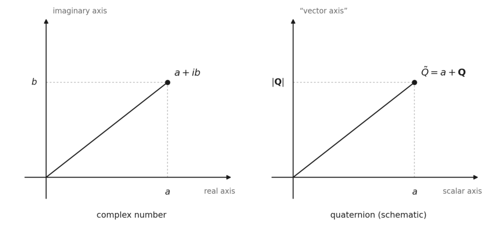
The figure is a mnemonic, not a diagram of the structure. A complex number splits into a real and an imaginary coordinate; a quaternion splits into a scalar and a vector part, and plotting the magnitude of that vector part on a single axis reproduces the right relationship for the norm, since

depends on Q only through its magnitude, exactly as the modulus of a complex number depends only on b.

Two things are hidden rather than simplified, and both matter.

The direction of Q is gone. Compressing three components onto one axis keeps the magnitude and discards everything else, and no amount of redrawing fixes this: adding a third axis would recover two of the three components and arbitrarily privilege them over the third. What is needed is not another axis but a change of kind — the vector part promoted to a genuine three-dimensional subspace, with the scalar carried as a fourth coordinate alongside it. That is a four-dimensional object, and it cannot be drawn.

And the non-commutativity is invisible. Nothing a two-dimensional picture can suggest reproduces the actual product, because the picture has no way to express that the order of multiplication changes the answer. The figure is authoritative on the norm, and on nothing else.

What the algebra is good for

The immediate application, and the one still in daily use, is rotation. Unit quaternions represent rotations in three-dimensional space without the degenerate configurations that afflict angle-based descriptions, and they compose by multiplication. Computer graphics, robotics and spacecraft attitude control all run on this.

But the property that matters for physics is the one that came out of the product above. In the vector calculus that replaced quaternions in the 1880s, the dot product and the cross product are two separate operations, defined independently, with no structural relation to each other. In quaternion algebra they are two parts of a single multiplication — and any product of two quaternions carrying vector parts necessarily generates both.

That is a statement about algebra, not about physics, and nothing here claims otherwise. But it is worth noticing that a formalism which cannot produce one without the other will behave differently, when applied to a physical problem, from one in which the two are separate by construction.

---

Sources

• W. R. Hamilton, “On quaternions,” Proc. R. Irish Acad., vol. 3, pp. 1–16, 1847.
• G. Frobenius, “Über lineare Substitutionen und bilineare Formen,” J. Reine Angew. Math., vol. 84, pp. 1–63, 1878.
• A. Gsponer and J.-P. Hurni, “The Physical Heritage of Sir W. R. Hamilton,” arXiv:math-ph/0201058.